9.9 Scattering from Hair
Human hair and animal fur can be modeled with a rough dielectric interface surrounding a pigmented translucent core. Reflectance at the interface is generally the same for all wavelengths and it is therefore wavelength-variation in the amount of light that is absorbed inside the hair that determines its color. While these scattering effects could be modeled using a combination of the DielectricBxDF and the volumetric scattering models from Chapters 11 and 14, not only would doing so be computationally expensive, requiring ray tracing within the hair geometry, but importance sampling the resulting model would be difficult. Therefore, this section introduces a specialized BSDF for hair and fur that encapsulates these lower-level scattering processes into a model that can be efficiently evaluated and sampled.
See Figure 9.39 for an example of the visual complexity of scattering in hair and a comparison to rendering using a conventional BRDF model with hair geometry.
9.9.1 Geometry
Before discussing the mechanisms of light scattering from hair, we will start by defining a few ways of measuring incident and outgoing directions at ray intersection points on hair. In doing so, we will assume that the hair BSDF is used with the Curve shape from Section 6.7, which allows us to make assumptions about the parameterization of the hair geometry. For the geometric discussion in this section, we will assume that the Curve variant corresponding to a flat ribbon that is always facing the incident ray is being used. However, in the BSDF model, we will interpret intersection points as if they were on the surface of the corresponding swept cylinder. If there is no interpenetration between hairs and if the hair’s width is not much larger than a pixel’s width, there is no harm in switching between these interpretations.
Throughout the implementation of this scattering model, we will find it useful to separately consider scattering in the longitudinal plane, effectively using a side view of the curve, and scattering in the azimuthal plane, considering the curve head-on at a particular point along it. To understand these parameterizations, first recall that Curves are parameterized such that the direction is along the length of the curve and spans its width. At a given , all the possible surface normals of the curve are given by the surface normals of the circular cross-section at that point. All of these normals lie in a plane that is called the normal plane (Figure 9.40).


We will find it useful to represent directions at a ray–curve intersection point with respect to coordinates that are defined with respect to the normal plane at the position where the ray intersected the curve. The angle is the longitudinal angle, which is the offset of the ray with respect to the normal plane (Figure 9.41(a)); ranges from to , where corresponds to a direction aligned with and corresponds to . As explained in Section 9.1.1, in pbrt’s regular BSDF coordinate system, is aligned with the axis, so given a direction in the BSDF coordinate system, we have , since the normal plane is perpendicular to .
In the BSDF coordinate system, the normal plane is spanned by the and coordinate axes. ( corresponds to for curves, which is always perpendicular to the curve’s , and is aligned with the ribbon normal.) The azimuthal angle is found by projecting a direction into the normal plane and computing its angle with the axis. It thus ranges from to (Figure 9.41(b)).
One more measurement with respect to the curve will be useful in the following. Consider incident rays with some direction : at any given parametric value, all such rays that intersect the curve can only possibly intersect one half of the circle swept along the curve (Figure 9.42). We will parameterize the circle’s diameter with the variable , where corresponds to the ray grazing the edge of the circle, and corresponds to hitting it edge-on. Because pbrt parameterizes curves with across the curve, we can compute .
Given the for a ray intersection, we can compute the angle between the surface normal of the inferred swept cylinder (which is by definition in the normal plane) and the direction , which we will denote by . (Note: this is unrelated to the notation used for floating-point error bounds in Section 6.8.) See Figure 9.42, which shows that .

9.9.2 Scattering from Hair
Geometric setting in hand, we will now turn to discuss the general scattering behaviors that give hair its distinctive appearance and some of the assumptions that we will make in the following.
Hair and fur have three main components:
- Cuticle: The outer layer, which forms the boundary with air. The cuticle’s surface is a nested series of scales at a slight angle to the hair surface.
- Cortex: The next layer inside the cuticle. The cortex generally accounts for around 90% of hair’s volume but less for fur. It is typically colored with pigments that mostly absorb light.
- Medulla: The center core at the middle of the cortex. It is larger and more significant in thicker hair and fur. The medulla is also pigmented. Scattering from the medulla is much more significant than scattering from the medium in the cortex.
For the following scattering model, we will make a few assumptions. (Approaches for relaxing some of them are discussed in the exercises at the end of this chapter.) First, we assume that the cuticle can be modeled as a rough dielectric cylinder with scales that are all angled at the same angle (effectively giving a nested series of cones; see Figure 9.43). We also treat the hair interior as a homogeneous medium that only absorbs light—scattering inside the hair is not modeled directly. (Chapters 11 and 14 have detailed discussion of light transport in participating media.)

We will also make the assumption that scattering can be modeled accurately by a BSDF—we model light as entering and exiting the hair at the same place. (A BSSRDF could certainly be used instead; the “Further Reading” section has pointers to work that has investigated that alternative.) Note that this assumption requires that the hair’s diameter be fairly small with respect to how quickly illumination changes over the surface; this assumption is generally fine in practice at typical viewing distances.

Incident light arriving at a hair may be scattered one or more times before leaving the hair; Figure 9.44 shows a few of the possible cases. We will use to denote the number of path segments it follows inside the hair before being scattered back out to air. We will sometimes refer to terms with a shorthand that describes the corresponding scattering events at the boundary: corresponds to , for reflection, is , for two transmissions is , is , and so forth.
In the following, we will find it useful to consider these scattering modes separately and so will write the hair BSDF as a sum over terms :
To make the scattering model evaluation and sampling easier, many hair scattering models factor into terms where one depends only on the angles and another on , the difference between and . This semi-separable model is given by:
where we have a longitudinal scattering function , an attenuation function , and an azimuthal scattering function . The division by cancels out the corresponding factor in the reflection equation.
In the following implementation, we will evaluate the first few terms of the sum in Equation (9.47) and then represent all higher-order terms with a single one. The pMax constant controls how many are evaluated before the switch-over.
The model implemented in the HairBxDF is parameterized by six values:
- h: the offset along the curve width where the ray intersected the oriented ribbon.
- eta: the index of refraction of the interior of the hair (typically, 1.55).
- sigma_a: the absorption coefficient of the hair interior, where distance is measured with respect to the hair cylinder’s diameter. (The absorption coefficient is introduced in Section 11.1.1.)
- beta_m: the longitudinal roughness of the hair, mapped to the range .
- beta_n: the azimuthal roughness, also mapped to .
- alpha: the angle at which the small scales on the surface of hair are offset from the base cylinder, expressed in degrees (typically, 2).
Beyond initializing corresponding member variables, the HairBxDF constructor performs some additional precomputation of values that will be useful for sampling and evaluation of the scattering model. The corresponding code will be added to the <<HairBxDF constructor implementation>> fragment in the following, closer to where the corresponding values are defined and used. Note that alpha is not stored in a member variable; it is used to compute a few derived quantities that will be, however.
We will start with the method that evaluates the BSDF.
There are a few quantities related to the directions and that are needed for evaluating the hair scattering model—specifically, the sine and cosine of the angle that each direction makes with the plane perpendicular to the curve, and the angle in the azimuthal coordinate system.
As explained in Section 9.9.1, is given by the component of in the BSDF coordinate system. Given , because , we know that must be positive, and so we can compute using the identity . The angle in the perpendicular plane can be computed with std::atan.
Equivalent code computes these values for wi.
With these values available, we will consider in turn the factors of the BSDF model—, , and —before returning to the completion of the f() method.
9.9.3 Longitudinal Scattering
defines the component of scattering related to the angles —longitudinal scattering. Longitudinal scattering is responsible for the specular lobe along the length of hair and the longitudinal roughness controls the size of this highlight. Figure 9.45 shows hair geometry rendered with three different longitudinal scattering roughnesses.
The mathematical details of the derivation of the scattering model are complex, so we will not include them here; as always, the “Further Reading” section has references to the details. The design goals of the model implemented here were that it be normalized (ensuring both energy conservation and no energy loss) and that it could be sampled directly. Although this model is not directly based on a physical model of how hair scatters light, it matches measured data well and has parametric control of roughness .
The model is:
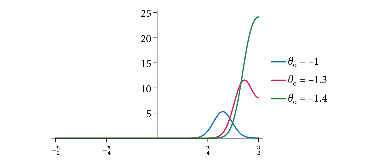
where is the modified Bessel function of the first kind and is the roughness variance. Figure 9.46 shows plots of .
This model is not numerically stable for low roughness variance values, so our implementation uses a different approach for that case that operates on the logarithm of before taking an exponent at the end. The v <= .1 test in the implementation below selects between the two formulations.
One challenge with this model is choosing a roughness to achieve a desired look. Here we have implemented a perceptually uniform mapping from roughness to where a roughness of 0 is nearly perfectly smooth and 1 is extremely rough. Different roughness values are used for different values of . For , roughness is reduced by an empirical factor that models the focusing of light due to refraction through the circular boundary of the hair. It is then increased for and subsequent terms, which models the effect of light spreading out after multiple reflections at the rough cylinder boundary in the interior of the hair.
9.9.4 Absorption in Fibers
The factor describes how the incident light is affected by each of the scattering modes . It incorporates two effects: Fresnel reflection and transmission at the hair–air boundary and absorption of light that passes through the hair (for ). Figure 9.47 has rendered images of hair with varying absorption coefficients, showing the effect of absorption. The function that we have implemented models all reflection and transmission at the hair boundary as perfect specular—a very different assumption than and (to come), which model glossy reflection and transmission. This assumption simplifies the implementation and gives reasonable results in practice (presumably in that the specular paths are, in a sense, averages over all the possible glossy paths).
We will start by finding the fraction of incident light that remains after a path of a single transmitted segment through the hair. To do so, we need to find the distance the ray travels until it exits the cylinder; the easiest way to do this is to compute the distances in the longitudinal and azimuthal projections separately.
To compute these distances, we need the transmitted angles of the ray , in the longitudinal and azimuthal planes, which we will denote by and , respectively. Application of Snell’s law using the hair’s index of refraction allows us to compute and .
For , although we could compute the transmitted direction from and then project into the normal plane, it is possible to compute directly using a modified index of refraction that accounts for the effect of the longitudinal angle on the refracted direction in the normal plane. The modified index of refraction is given by
Given , we can compute the refracted direction directly in the normal plane. Since , we can apply Snell’s law to compute .

If we consider the azimuthal projection of the transmitted ray in the normal plane, we can see that the segment makes the same angle with the circle normal at both of its endpoints (Figure 9.48). If we denote the total length of the segment by , then basic trigonometry tells us that , assuming a unit radius circle.

Now considering the longitudinal projection, we can see that the distance that a transmitted ray travels before exiting is scaled by a factor of as it passes through the cylinder (Figure 9.49). Putting these together, the total segment length in terms of the hair diameter is
Given the segment length and the medium’s absorption coefficient, the fraction of light transmitted can be computed using Beer’s law, which is introduced in Section 11.2. Because the HairBxDF defined to be measured with respect to the hair diameter (so that adjusting the hair geometry’s width does not completely change its color), we do not consider the hair cylinder diameter when we apply Beer’s law, and the fraction of light remaining at the end of the segment is given by
Given a single segment’s transmittance, we can now describe the function that evaluates the full function. Ap() returns an array with the values of up to and a final value that is the sum of attenuations for all the higher-order scattering terms.
For the term, corresponding to light that reflects at the cuticle, the Fresnel reflectance at the air–hair boundary gives the fraction of light that is reflected. We can find the cosine of the angle between the surface normal and the direction vector with angles and in the hair coordinate system by .
For the term, , we have two factors, accounting for transmission into and out of the cuticle boundary, and a single factor for one transmission path through the hair.

The term has one more reflection event, reflecting light back into the hair, and then a second transmission term. Since we assume perfect specular reflection at the cuticle boundary, both segments inside the hair make the same angle with the circle’s normal (Figure 9.50). From this, we can see that both segments must have the same length (and so forth for subsequent segments). In general, for ,
After pMax, a final term accounts for all further orders of scattering. The sum of the infinite series of remaining terms can fortunately be found in closed form, since both and :
9.9.5 Azimuthal Scattering

Finally, we will model the component of scattering dependent on the angle . We will do this work entirely in the normal plane. The azimuthal scattering model is based on first computing a new azimuthal direction assuming perfect specular reflection and transmission and then defining a distribution of directions around this central direction, where increasing roughness gives a wider distribution. Therefore, we will first consider how an incident ray is deflected by specular reflection and transmission in the normal plane; Figure 9.51 illustrates the cases for the first two values of .
Following the reasoning from Figure 9.51, we can derive the function , which gives the net change in azimuthal direction:
(Recall that and are derived from .) Figure 9.52 shows a plot of this function for .

Now that we know how to compute new angles in the normal plane after specular transmission and reflection, we need a way to represent surface roughness, so that a range of directions centered around the specular direction can contribute to scattering. The logistic distribution provides a good option: it is a generally useful one for rendering, since it has a similar shape to the Gaussian, while also being normalized and integrable in closed form (unlike the Gaussian); see Section B.2.5 for more information.

In the following, we will find it useful to define a normalized logistic function over a range ; we will call this the trimmed logistic, .
Figure 9.53 shows plots of the trimmed logistic distribution for a few values of .
Now we have the pieces to be able to implement the azimuthal scattering distribution. The Np() function computes the term, finding the angular difference between and and evaluating the azimuthal distribution with that angle.
The difference between and may be outside the range we have defined the logistic over, , so we rotate around the circle as needed to get the value to the right range. Because dphi never gets too far out of range for the small used here, we use the simple approach of adding or subtracting as needed.
As with the longitudinal roughness, it is helpful to have a roughly perceptually linear mapping from azimuthal roughness to the logistic scale factor .

Figure 9.54 shows polar plots of azimuthal scattering for the term, , with a fairly low roughness. The scattering distributions for the two different points on the curve’s width are quite different. Because we expect the hair width to be roughly pixel-sized, many rays per pixel are needed to resolve this variation well.
9.9.6 Scattering Model Evaluation
We now have almost all the pieces we need to be able to evaluate the model. The last detail is to account for the effect of scales on the hair surface (recall Figure 9.43). Suitable adjustments to work well to model this characteristic of hair.
For the term, adding the angle to can model the effect of evaluating the hair scattering model with respect to the surface normal of a scale. We can then go ahead and evaluate with this modification to . For , we have to account for two transmission events through scales. Rotating by in the opposite direction approximately compensates. (Because the refraction angle is nonlinear with respect to changes in normal orientation, there is some error in this approximation, though the error is low for the typical case of small values of .) has a reflection term inside the hair; a rotation by compensates for the overall effect.
The effects of these shifts are that the primary reflection lobe is offset to be above the perfect specular direction and the secondary lobe is shifted below it. Together, these lead to two distinct specular highlights of different colors, since is not affected by the hair’s color, while picks up the hair color due to absorption. This effect can be seen in human hair and is evident in the images in Figure 9.45, for example.
Because we only need the sine and cosine of the angle to evaluate , we can use the trigonometric identities
to efficiently compute the rotated angles without needing to evaluate any additional trigonometric functions. The HairBxDF constructor therefore precomputes and for . These values can be computed particularly efficiently using trigonometric double angle identities: and .
Evaluating the model is now mostly just a matter of calling functions that have already been defined and summing the individual terms .
The rotations that account for the effect of scales are implemented using the trigonometric identities listed above. Here is the code for the case, where is rotated by . The remaining cases follow the same structure. (The rotation is by for and by for .)
When is nearly parallel with the hair, the scale adjustment may give a slightly negative value for —effectively, in this case, it represents a that is slightly greater than , the maximum expected value of in the hair coordinate system. This angle is equivalent to , and , so we can easily handle that here.
A final term accounts for all higher-order scattering inside the hair. We just use a uniform distribution for the azimuthal distribution; this is a reasonable choice, as the direction offsets from for generally have wide variation and the final term generally represents less than 15% of the overall scattering, so little error is introduced in the final result.
A Note on Reciprocity
Although we included reciprocity in the properties of physically valid BRDFs in Section 4.3.1, the model we have implemented in this section is, unfortunately, not reciprocal. An immediate issue is that the rotation for hair scales is applied only to . However, there are more problems: first, all terms that involve transmission are not reciprocal since the transmission terms use values based on , which itself only depends on . Thus, if and are interchanged, a completely different is computed, which in turn leads to different and values, which in turn give different values from the and functions. In practice, however, we have not observed artifacts in images from these shortcomings.
9.9.7 Sampling
Being able to generate sampled directions and compute the PDF for sampling a given direction according to a distribution that is similar to the overall BSDF is critical for efficient rendering, especially at low roughnesses, where the hair BSDF varies rapidly as a function of direction. In the approach implemented here, samples are generated with a two-step process: first we choose a term to sample according to a probability based on each term’s function value, which gives its contribution to the overall scattering function. Then, we find a direction by sampling the corresponding and terms. Fortunately, both the and terms of the hair BSDF can be sampled perfectly, leaving us with a sampling scheme that exactly matches the PDF of the full BSDF.
We will first define the ApPDF() method, which returns a discrete PDF with probabilities for sampling each term according to its contribution relative to all the terms, given .
The method starts by computing the values of for cosTheta_o. We are able to reuse some previously defined fragments to make this task easier.
Next, the spectral values are converted to scalars using their luminance and these values are normalized to make a proper PDF.
With these preliminaries out of the way, we can now implement the Sample_f() method.
Given the PDF over terms, a call to SampleDiscrete() takes care of choosing one. Because we only need to generate one sample from the PDF’s distribution, the work to compute an explicit CDF array (for example, by using PiecewiseConstant1D) is not worthwhile. Note that we take advantage of SampleDiscrete()’s optional capability of returning a fresh uniform random sample, overwriting the value in uc. This sample value will be used shortly for sampling .
We can now sample the corresponding term given to find . The derivation of this sampling method is fairly involved, so we will include neither the derivation nor the implementation here. This fragment, <<Sample to compute >>, consumes both of the sample values u[0] and u[1] and initializes variables sinTheta_i and cosTheta_i according to the sampled direction.
Next we will sample the azimuthal distribution . For terms up to , we take a sample from the logistic distribution centered around the exit direction given by . For the last term, we sample from a uniform distribution.
Given and , we can compute the sampled direction wi. The math is similar to that used in the SphericalDirection() function, but with two important differences. First, because here is measured with respect to the plane perpendicular to the cylinder rather than the cylinder axis, we need to compute for the coordinate with respect to the cylinder axis instead of . Second, because the hair shading coordinate system’s coordinates are oriented with respect to the axis, the order of dimensions passed to the Vector3f constructor is adjusted correspondingly, since the direction returned from Sample_f() should be in the BSDF coordinate system.
Because we could sample directly from the and distributions, the overall PDF is
where are the normalized PDF terms. Note that must be shifted to account for hair scales when evaluating the PDF; this is done in the same way (and with the same code fragment) as with BSDF evaluation.
The HairBxDF::PDF() method performs the same computation and therefore the implementation is not included here.
9.9.8 Hair Absorption Coefficients
The color of hair is determined by how pigments in the cortex absorb light, which in turn is described by the normalized absorption coefficient where distance is measured in terms of the hair diameter. If a specific hair color is desired, there is a non-obvious relationship between the normalized absorption coefficient and the color of hair in a rendered image. Not only does changing the spectral values of the absorption coefficient have an unpredictable connection to the appearance of a single hair, but multiple scattering between collections of many hairs has a significant effect on each one’s apparent color. Therefore, pbrt provides implementations of two more intuitive ways to specify hair color.
The first is based on the fact that the color of human hair is determined by the concentration of two pigments. The concentration of eumelanin is the primary factor that causes the difference between black, brown, and blonde hair. (Black hair has the most eumelanin and blonde hair has the least. White hair has none.) The second pigment, pheomelanin, causes hair to be orange or red. The HairBxDF class provides a convenience method that computes an absorption coefficient using the product of user-supplied pigment concentrations and absorption coefficients of the pigments.
Eumelanin concentrations of roughly 8, 1.3, and 0.3 give reasonable representations of black, brown, and blonde hair, respectively. Accurately rendering light-colored hair requires simulating many interreflections of light, however; see Figure 9.55.
It is also sometimes useful to specify the desired hair color directly; the SigmaAFromReflectance() method, not included here, is based on a precomputed fit of absorption coefficients to scattered hair color.