11.2 Transmittance

The scattering processes in Section 11.1 are all specified in terms of their local effect at points in space. However, in rendering, we are usually interested in their aggregate effects on radiance along a ray, which usually requires transforming the differential equations to integral equations that can be solved using Monte Carlo. The reduction in radiance between two points on a ray due to extinction is a quantity that will often be useful; for example, we will need to estimate this value to compute the attenuated radiance from a light source that is incident at a point on a surface in scenes with participating media.

Given the attenuation coefficient sigma Subscript normal t , the differential equation that describes extinction,

StartFraction normal d upper L Subscript normal o Baseline left-parenthesis normal p Subscript Baseline comma omega Subscript Baseline right-parenthesis Over normal d t EndFraction equals minus sigma Subscript normal t Baseline left-parenthesis normal p Subscript Baseline comma omega Subscript Baseline right-parenthesis upper L Subscript normal i Baseline left-parenthesis normal p Subscript Baseline comma minus omega Subscript Baseline right-parenthesis comma

can be solved to find the beam transmittance upper T Subscript normal r , which gives the fraction of radiance that is transmitted between two points:
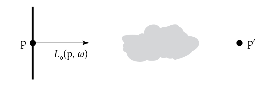
upper T Subscript normal r Baseline left-parenthesis normal p Subscript Baseline right-arrow normal p Superscript prime Baseline right-parenthesis equals normal e Superscript minus integral Subscript 0 Superscript d Baseline sigma Super Subscript normal t Superscript left-parenthesis normal p Super Subscript Superscript plus t omega Super Subscript Superscript comma omega Super Subscript Superscript right-parenthesis normal d t Baseline comma

where d equals double-vertical-bar normal p Subscript Baseline minus normal p prime double-vertical-bar is the distance between normal p Subscript and normal p prime , and omega Subscript is the normalized direction vector between them. Note that the transmittance is always between 0 and 1. Thus, if exitant radiance from a point normal p Subscript on a surface in a given direction omega Subscript is given by upper L Subscript normal o Superscript Baseline left-parenthesis normal p Subscript Baseline comma omega Subscript Baseline right-parenthesis , then after accounting for extinction the incident radiance at another point normal p prime in direction minus omega Subscript  is

upper T Subscript r Baseline left-parenthesis normal p Subscript Baseline right-arrow normal p Superscript prime Baseline right-parenthesis upper L Subscript normal o Superscript Baseline left-parenthesis normal p Subscript Baseline comma omega Subscript Baseline right-parenthesis period

This idea is illustrated in Figure 11.9.

Figure 11.9: The beam transmittance upper T Subscript r Baseline left-parenthesis normal p Subscript Baseline right-arrow normal p prime right-parenthesis gives the fraction of light transmitted from one point to another, accounting for absorption and out scattering, but ignoring emission and in scattering. Given exitant radiance at a point normal p Subscript in direction omega Subscript (e.g., reflected radiance from a surface), the radiance visible at another point normal p prime along the ray is upper T Subscript r Baseline left-parenthesis normal p Subscript Baseline right-arrow normal p Superscript prime Baseline right-parenthesis upper L Subscript normal o Superscript Baseline left-parenthesis normal p Subscript Baseline comma omega Subscript Baseline right-parenthesis .

Not only is transmittance useful for modeling the attenuation of light within participating media, but accounting for transmittance along shadow rays makes it possible to accurately model shadowing on surfaces due to the effect of media; see Figure 11.10.

Figure 11.10: Shadow-Casting Volumetric Bunny. The bunny, which is modeled entirely with participating media, casts a shadow on the ground plane because it attenuates light from the sun (which is to the left) on its way to the ground. (Bunny courtesy of the Stanford Computer Graphics Laboratory; volumetric enhancement courtesy of the OpenVDB sample model repository.)

Two useful properties of beam transmittance are that transmittance from a point to itself is 1, upper T Subscript r Baseline left-parenthesis normal p Subscript Baseline right-arrow normal p Subscript Baseline right-parenthesis equals 1 , and in a vacuum sigma Subscript normal t Baseline equals 0 and so upper T Subscript r Baseline left-parenthesis normal p Subscript Baseline right-arrow normal p prime right-parenthesis equals 1 for all normal p prime . Furthermore, if the attenuation coefficient satisfies the directional symmetry sigma Subscript normal t Baseline left-parenthesis omega Subscript Baseline right-parenthesis equals sigma Subscript normal t Baseline left-parenthesis minus omega Subscript Baseline right-parenthesis or does not vary with direction omega Subscript and only varies as a function of position, then the transmittance between two points is the same in both directions:

upper T Subscript r Baseline left-parenthesis normal p Subscript Baseline right-arrow normal p Superscript prime Baseline right-parenthesis equals upper T Subscript r Baseline left-parenthesis normal p prime right-arrow normal p Subscript Baseline right-parenthesis period

This property follows directly from Equation (11.5).

Figure 11.11: A useful property of beam transmittance is that it is multiplicative: the transmittance between points normal p Subscript and normal p double-prime on a ray like the one shown here is equal to the transmittance from normal p Subscript to normal p prime times the transmittance from normal p prime to normal p double-prime for all points normal p prime between normal p Subscript and  normal p double-prime .

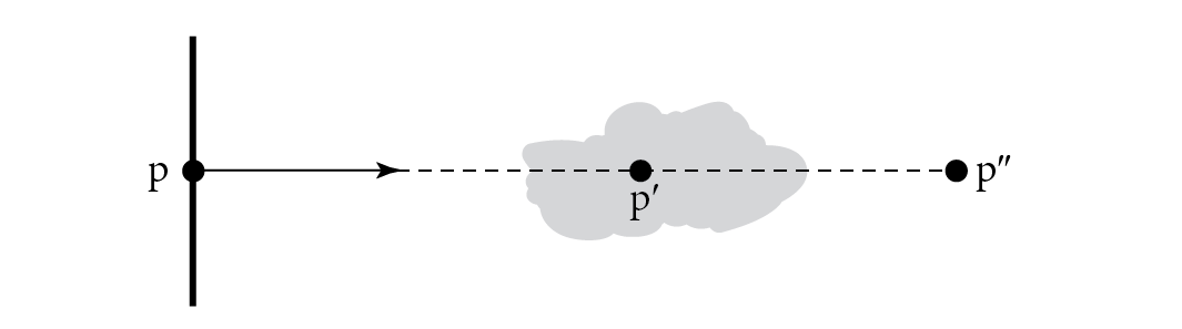
Another important property, true in all media, is that transmittance is multiplicative along points on a ray:

upper T Subscript r Baseline left-parenthesis normal p Subscript Baseline right-arrow normal p Superscript double-prime Baseline right-parenthesis equals upper T Subscript r Baseline left-parenthesis normal p Subscript Baseline right-arrow normal p Superscript prime Baseline right-parenthesis upper T Subscript r Baseline left-parenthesis normal p prime right-arrow normal p Superscript double-prime Baseline right-parenthesis comma

for all points normal p prime between normal p Subscript and normal p double-prime (Figure 11.11). This property is useful for volume scattering implementations, since it makes it possible to incrementally compute transmittance at multiple points along a ray: transmittance from the origin to a point upper T Subscript r Baseline left-parenthesis normal o right-arrow normal p Subscript Baseline right-parenthesis can be computed by taking the product of transmittance to a previous point upper T Subscript r Baseline left-parenthesis normal o right-arrow normal p prime right-parenthesis and the transmittance of the segment between the previous and the current point upper T Subscript r Baseline left-parenthesis normal p prime right-arrow normal p Subscript Baseline right-parenthesis .

The negated exponent in the definition of upper T Subscript r in Equation (11.5) is called the optical thickness between the two points. It is denoted by the symbol tau :

tau left-parenthesis normal p Subscript Baseline right-arrow normal p Superscript prime Baseline right-parenthesis equals integral Subscript 0 Superscript d Baseline sigma Subscript normal t Baseline left-parenthesis normal p Subscript Baseline plus t omega Subscript Baseline comma omega Subscript Baseline right-parenthesis normal d t period

In a homogeneous medium, sigma Subscript normal t is a constant, so the integral that defines tau is trivially evaluated, giving Beer’s law:

upper T Subscript r Baseline left-parenthesis normal p Subscript Baseline right-arrow normal p Superscript prime Baseline right-parenthesis equals normal e Superscript minus sigma Super Subscript normal t Superscript d Baseline period

It may appear that a straightforward application of Monte Carlo could be used to compute the beam transmittance in inhomogeneous media. Equation (11.5) consists of a 1D integral over a ray’s parametric t position that is then exponentiated; given a method to sample distances along the ray t prime according to some distribution p , one could evaluate the estimator:

normal e Superscript minus integral Subscript 0 Superscript d Baseline sigma Super Subscript normal t Superscript left-parenthesis normal p Super Subscript Superscript plus t omega Super Subscript Superscript comma omega Super Subscript Superscript right-parenthesis normal d t Baseline almost-equals normal e Superscript minus left-bracket StartFraction sigma Super Subscript normal t Superscript left-parenthesis normal p Super Subscript Superscript plus t prime omega Super Subscript Superscript comma omega Super Subscript Superscript right-parenthesis Over p left-parenthesis t Super Superscript prime Superscript right-parenthesis EndFraction right-bracket Baseline period

However, even if the estimator in square brackets is an unbiased estimator of the optical thickness along the ray, the estimate of transmittance is not unbiased and will actually underestimate its value: upper E left-bracket normal e Superscript negative upper X Baseline right-bracket not-equals normal e Superscript minus upper E left-bracket upper X right-bracket . (This state of affairs is explained by Jensen’s inequality and the fact that normal e Superscript negative x is a convex function.)

The error introduced by estimators of the form of Equation (11.8) decreases as error in the estimate of the beam transmittance decreases. For many applications, this error may be acceptable—it is still widespread practice in graphics to estimate tau in some manner, e.g., via a Riemann sum, and then to compute the transmittance that way. However, it is possible to derive an alternative equation for transmittance that allows unbiased estimation; that is the approach used in pbrt.

First, we will consider the change in radiance between two points normal p Subscript and normal p prime along the ray. Integrating Equation (11.4) and dropping the directional dependence of sigma Subscript normal t for notational simplicity, we can find that

integral Subscript 0 Superscript d Baseline StartFraction normal d upper L left-parenthesis normal p Subscript Baseline plus t omega Subscript Baseline right-parenthesis Over normal d t EndFraction normal d t equals upper L left-parenthesis normal p Superscript prime Baseline right-parenthesis minus upper L left-parenthesis normal p Subscript Baseline right-parenthesis equals integral Subscript 0 Superscript d Baseline minus sigma Subscript normal t Baseline left-parenthesis normal p Subscript Baseline plus t omega Subscript Baseline right-parenthesis upper L left-parenthesis normal p Subscript Baseline plus t omega Subscript Baseline right-parenthesis normal d t comma

where, as before, d is the distance between normal p Subscript and normal p prime and omega Subscript is the normalized vector from normal p Subscript to  normal p prime .

The transmittance is the fraction of the original radiance, and so upper T Subscript normal r Baseline left-parenthesis normal p Subscript Baseline right-arrow normal p prime right-parenthesis equals upper L left-parenthesis normal p prime right-parenthesis slash upper L left-parenthesis normal p Subscript Baseline right-parenthesis . Thus, if we divide Equation (11.9) by upper L left-parenthesis normal p Subscript Baseline right-parenthesis and rearrange terms, we can find that

upper T Subscript normal r Baseline left-parenthesis normal p Subscript Baseline right-arrow normal p Superscript prime Baseline right-parenthesis equals 1 minus integral Subscript 0 Superscript d Baseline sigma Subscript normal t Baseline left-parenthesis normal p Subscript Baseline plus t omega Subscript Baseline right-parenthesis upper T Subscript normal r Baseline left-parenthesis normal p Subscript Baseline plus t omega Subscript Baseline right-arrow normal p Superscript prime Baseline right-parenthesis normal d t period

We have found ourselves with transmittance defined recursively in terms of an integral that includes transmittance in the integrand; although this may seem to be making the problem more complex than it was before, this definition makes it possible to apply Monte Carlo to the integral and to compute unbiased estimates of transmittance. However, it is difficult to sample this integrand well; in practice, estimates of it will have high variance. Therefore, the following section will introduce an alternative formulation of it that is amenable to sampling and makes a number of efficient solution techniques possible.

11.2.1 Null Scattering

The key idea that makes it possible to derive a more easily sampled transmittance integral is an approach known as null scattering. Null scattering is a mathematical formalism that can be interpreted as introducing an additional type of scattering that does not correspond to any type of physical scattering process but is specified so that it has no effect on the distribution of light. In doing so, null scattering makes it possible to treat inhomogeneous media as if they were homogeneous, which makes it easier to apply sampling algorithms to inhomogeneous media. (In Chapter 14, we will see that it is a key foundation for volumetric light transport algorithms beyond transmittance estimation.)

Figure 11.12: If the null-scattering coefficient is defined using a majorant sigma Subscript normal m normal a normal j as in Equation (11.11), then it can be interpreted as taking (a) an inhomogeneous medium (dark circles) and (b) filling it with fictitious particles (light circles) until it reaches a uniform density.

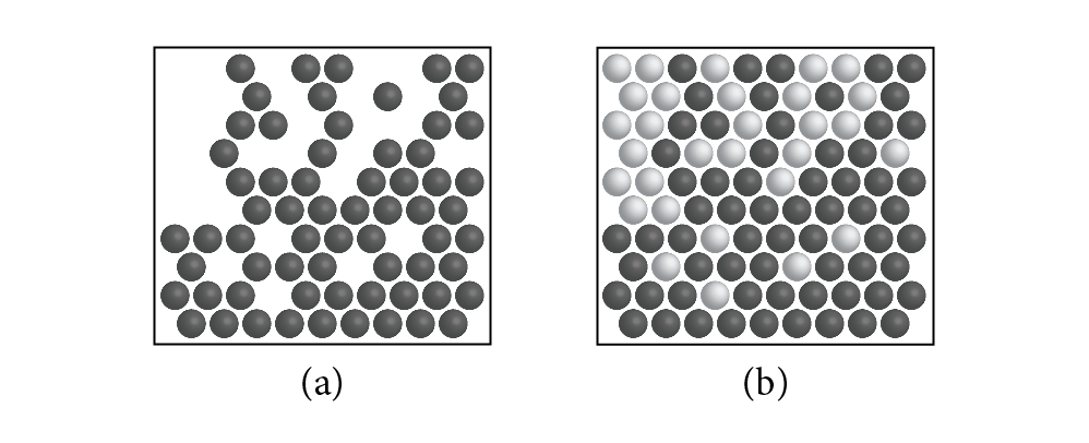
We will start by defining the null-scattering coefficient sigma Subscript normal n . Similar to the other scattering coefficients, it gives the probability of a null-scattering event per unit distance traveled in the medium. Here, we will define sigma Subscript normal n Baseline left-parenthesis normal p Subscript Baseline right-parenthesis via a constant majorant sigma Subscript normal m normal a normal j that is greater than or equal to sigma Subscript normal a Baseline plus sigma Subscript normal s at all points in the medium:

sigma Subscript normal n Baseline left-parenthesis normal p Subscript Baseline comma omega Subscript Baseline right-parenthesis equals sigma Subscript normal m normal a normal j Baseline minus sigma Subscript normal t Baseline left-parenthesis normal p Subscript Baseline comma omega Subscript Baseline right-parenthesis period

Thus, the total scattering coefficient sigma Subscript normal a Baseline plus sigma Subscript normal s Baseline plus sigma Subscript normal n Baseline equals sigma Subscript normal m normal a normal j is uniform throughout the medium. (This idea is illustrated in Figure 11.12.)

With this definition of sigma Subscript normal n , we can rewrite Equation (11.4) in terms of the majorant and the null-scattering coefficient:

StartFraction normal d upper L Subscript normal o Baseline left-parenthesis normal p Subscript Baseline comma omega Subscript Baseline right-parenthesis Over normal d t EndFraction equals minus left-parenthesis sigma Subscript normal m normal a normal j Baseline minus sigma Subscript normal n Baseline left-parenthesis normal p Subscript Baseline comma omega Subscript Baseline right-parenthesis right-parenthesis upper L Subscript normal i Baseline left-parenthesis normal p Subscript Baseline comma minus omega Subscript Baseline right-parenthesis period

We will not include the full derivation here, but just as with Equation (11.10), this equation can be integrated over the segment of a ray and divided by the initial radiance upper L left-parenthesis normal p Subscript Baseline right-parenthesis to find an equation for the transmittance. The result is:

upper T Subscript normal r Baseline left-parenthesis normal p Subscript Baseline right-arrow normal p Superscript prime Baseline right-parenthesis equals normal e Superscript minus sigma Super Subscript normal m normal a normal j Superscript d Baseline plus integral Subscript 0 Superscript d Baseline normal e Superscript minus sigma Super Subscript normal m normal a normal j Superscript t Baseline sigma Subscript normal n Baseline left-parenthesis normal p Subscript Baseline plus t omega Subscript Baseline right-parenthesis upper T Subscript normal r Baseline left-parenthesis normal p Subscript Baseline plus t omega Subscript Baseline right-arrow normal p Superscript prime Baseline right-parenthesis normal d t period

Note that with this expression of transmittance and a homogeneous medium, sigma Subscript normal n Baseline equals 0 and the integral disappears. The first term then corresponds to Beer’s law. For inhomogeneous media, the first term can be seen as computing an underestimate of the true transmittance, where the integral then accounts for the rest of it.

To compute Monte Carlo estimates of Equation (11.13), we would like to sample a distance t prime from some distribution that is proportional to the integrand and then apply the regular Monte Carlo estimator. A convenient sampling distribution is the probability density function (PDF) of the exponential distribution that is derived in Section A.4.2. In this case, the PDF associated with normal e Superscript minus sigma Super Subscript normal m normal a normal j Superscript t is

p Subscript normal m normal a normal j Baseline left-parenthesis t right-parenthesis equals sigma Subscript normal m normal a normal j Baseline normal e Superscript minus sigma Super Subscript normal m normal a normal j Superscript t

and a corresponding sampling recipe is available via the SampleExponential() function.

Because p Subscript normal m normal a normal j is nonzero over the range left-bracket 0 comma normal infinity right-parenthesis , the sampling algorithm will sometimes generate samples t prime greater-than d , which may seem to be undesirable. However, although we could define a PDF for the exponential function limited to left-bracket 0 comma d right-bracket , sampling from p Subscript normal m normal a normal j leads to a simple way to terminate the recursive evaluation of transmittance. To see why, consider rewriting the second term of Equation (11.13) as the sum of two integrals that cover the range left-bracket 0 comma normal infinity right-parenthesis :

integral Subscript 0 Superscript d Baseline normal e Superscript minus sigma Super Subscript normal m normal a normal j Superscript t Baseline sigma Subscript normal n Baseline left-parenthesis normal p Subscript Baseline plus t omega Subscript Baseline right-parenthesis upper T Subscript normal r Baseline left-parenthesis normal p Subscript Baseline plus t omega Subscript Baseline right-arrow normal p Superscript prime Baseline right-parenthesis normal d t plus integral Subscript d Superscript normal infinity Baseline 0 normal d t period

If the Monte Carlo estimator is applied to this sum, we can see that the value of t prime with respect to d determines which integrand is evaluated and thus that sampling t prime greater-than d can be conveniently interpreted as a condition for ending the recursive estimation of Equation (11.13).

Given the decision to sample from p Subscript normal m normal a normal j , perhaps the most obvious approach for estimating the value of Equation (11.13) is to sample t prime in this way and to directly apply the Monte Carlo estimator, which gives

upper T Subscript normal r Baseline left-parenthesis normal p Subscript Baseline right-arrow normal p prime right-parenthesis almost-equals normal e Superscript minus sigma Super Subscript normal m normal a normal j Superscript d Baseline plus StartLayout Enlarged left-brace 1st Row 1st Column StartFraction sigma Subscript normal n Baseline left-parenthesis normal p Subscript Baseline plus t prime omega Subscript Baseline right-parenthesis Over sigma Subscript normal m normal a normal j Baseline EndFraction upper T Subscript normal r Baseline left-parenthesis normal p Subscript Baseline plus t prime omega Subscript Baseline right-arrow normal p prime right-parenthesis 2nd Column t prime less-than d 2nd Row 1st Column 0 2nd Column otherwise period EndLayout

This estimator is known as the next-flight estimator. It has the advantage that it has zero variance for homogeneous media, although interestingly it is often not as efficient as other estimators for inhomogeneous media.

Other estimators randomly choose between the two terms of Equation (11.13) and only evaluate one of them. If we define p Subscript normal e as the discrete probability of evaluating the first term, transmittance can be estimated by

StartLayout 1st Row 1st Column upper T Subscript normal r Baseline left-parenthesis normal p Subscript Baseline right-arrow normal p prime right-parenthesis almost-equals StartLayout Enlarged left-brace 1st Row 1st Column StartFraction normal e Superscript minus sigma Super Subscript normal m normal a normal j Superscript d Baseline Over p Subscript normal e Baseline EndFraction 2nd Column with probability p Subscript normal e Baseline 2nd Row 1st Column StartFraction 1 Over 1 minus p Subscript normal e Baseline EndFraction integral Subscript 0 Superscript d Baseline normal e Superscript minus sigma Super Subscript normal m normal a normal j Superscript t Baseline sigma Subscript normal n Baseline left-parenthesis normal p Subscript Baseline plus t omega Subscript Baseline right-parenthesis upper T Subscript normal r Baseline left-parenthesis normal p Subscript Baseline plus t omega Subscript Baseline right-arrow normal p prime right-parenthesis normal d t 2nd Column otherwise period EndLayout 2nd Row 1st Column Blank 2nd Column Blank EndLayout

The ratio tracking estimator is the result from setting p Subscript normal e Baseline equals normal e Superscript minus sigma Super Subscript normal m normal a normal j Superscript d . Then, the first case of Equation (11.16) yields a value of 1. We can further combine the choice between the two cases with sampling t prime using the fact that the probability that t prime greater-than d is equal to normal e Superscript minus sigma Super Subscript normal m normal a normal j Superscript d . (This can be seen using p Subscript normal m normal a normal j ’s cumulative distribution function (CDF), Equation (A.17).) After simplifying, the resulting estimator works out to be:

upper T Subscript normal r Baseline left-parenthesis normal p Subscript Baseline right-arrow normal p prime right-parenthesis almost-equals StartLayout Enlarged left-brace 1st Row 1st Column 1 2nd Column t prime greater-than d 2nd Row 1st Column StartFraction sigma Subscript normal n Baseline left-parenthesis normal p Subscript Baseline plus t prime omega Subscript Baseline right-parenthesis Over sigma Subscript normal m normal a normal j Baseline EndFraction upper T Subscript normal r Baseline left-parenthesis normal p Subscript Baseline plus t prime omega Subscript Baseline right-arrow normal p prime right-parenthesis 2nd Column otherwise period EndLayout

If the recursive evaluations are expanded out, ratio tracking leads to an estimator of the form

upper T Subscript normal r Baseline left-parenthesis normal p Subscript Baseline right-arrow normal p Superscript prime Baseline right-parenthesis almost-equals product Underscript i Overscript n Endscripts StartFraction sigma Subscript normal n Baseline left-parenthesis p plus t Subscript i Baseline omega Subscript Baseline right-parenthesis Over sigma Subscript normal m normal a normal j Baseline EndFraction comma

where t Subscript i are the series of t values that are sampled from p Subscript normal m normal a normal j and where successive t Subscript i values are sampled starting from the previous one until one is sampled past the endpoint. Ratio tracking is the technique that is implemented to compute transmittance in pbrt’s light transport routines in Chapter 14.

A disadvantage of ratio tracking is that it continues to sample the medium even after the transmittance has become very small. Russian roulette can be used to terminate recursive evaluation to avoid this problem. If the Russian roulette termination probability at each sampled point is set to be equal to the ratio of sigma Subscript normal n and sigma Subscript normal m normal a normal j , then the scaling cancels and the estimator becomes

upper T Subscript normal r Baseline left-parenthesis normal p Subscript Baseline right-arrow normal p prime right-parenthesis almost-equals StartLayout Enlarged left-brace 1st Row 1st Column 1 2nd Column t prime greater-than d 2nd Row 1st Column upper T Subscript normal r Baseline left-parenthesis normal p Subscript Baseline plus t prime omega Subscript Baseline right-arrow normal p prime right-parenthesis 2nd Column t prime less-than-or-equal-to d and with probability StartFraction sigma Subscript normal n Baseline left-parenthesis normal p Subscript Baseline plus t prime omega Subscript Baseline right-parenthesis Over sigma Subscript normal m normal a normal j Baseline EndFraction 3rd Row 1st Column 0 2nd Column otherwise period EndLayout

Thus, recursive estimation of transmittance continues either until termination due to Russian roulette or until the sampled point is past the endpoint. This approach is the track-length transmittance estimator, also known as delta tracking.

A physical interpretation of delta tracking is that it randomly decides whether the ray interacts with a true particle or a fictitious particle at each scattering event. Interactions with fictitious particles (corresponding to null scattering) are ignored and the algorithm continues, restarting from the sampled point. Interactions with true particles cause extinction, in which case 0 is returned. If a ray makes it through the medium without extinction, the value 1 is returned.

Delta tracking can also be used to sample positions t along a ray with probability proportional to sigma Subscript normal t Baseline left-parenthesis t right-parenthesis upper T Subscript normal r Baseline left-parenthesis t right-parenthesis . The algorithm is given by the following pseudocode, which assumes that the function u() generates a uniform random number between 0 and 1 and where the recursion has been transformed into a loop:

optional<Point> DeltaTracking(Point p, Vector w, Float sigma_maj, Float d) { Float t = SampleExponential(u(), sigma_maj); while (t < d) { Float sigma_n = /* evaluate sigma_n at p + t * w */; if (u() < sigma_n / sigma_maj) t += SampleExponential(u(), sigma_maj); else return p + t * w; } return {}; /* no sample before d */ }