6.7 Curves

While triangles or bilinear patches can be used to represent thin shapes for modeling fine geometry like hair, fur, or fields of grass, it is worthwhile to have a specialized Shape in order to more efficiently render these sorts of objects, since many individual instances of them are often present. The Curve shape, introduced in this section, represents thin geometry modeled with cubic Bézier curves, which are defined by four control points, , , , and . The Bézier spline passes through the first and last control points. Points along it are given by the polynomial

(See Figure 6.29.) Curves specified using another basis (e.g., Hermite splines or b-splines) must therefore be converted to the Bézier basis to be used with this Shape.

The Curve shape is defined by a 1D Bézier curve along with a width that is linearly interpolated from starting and ending widths along its extent. Together, these define a flat 2D surface (Figure 6.30). ^† It is possible to directly intersect rays with this representation without tessellating it, which in turn makes it possible to efficiently render smooth curves without using too much storage.

Figure 6.31 shows a bunny model with fur modeled with over one million Curves.

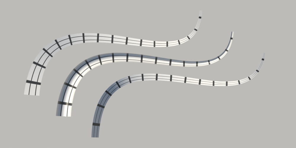
There are three types of curves that the Curve shape can represent, shown in Figure 6.32.

• Flat: Curves with this representation are always oriented to face the ray being intersected with them; they are useful for modeling fine swept cylindrical shapes like hair or fur.
• Cylinder: For curves that span a few pixels on the screen (like spaghetti seen from not too far away), the Curve shape can compute a shading normal that makes the curve appear to actually be a cylinder.
• Ribbon: This variant is useful for modeling shapes that do not actually have a cylindrical cross section (such as a blade of grass).

The CurveType enumerator records which of them a given Curve instance models.

The flat and cylinder curve variants are intended to be used as convenient approximations of deformed cylinders. It should be noted that intersections found with respect to them do not correspond to a physically realizable 3D shape, which can potentially lead to minor inconsistencies when taking a scene with true cylinders as a reference.

Given a curve specified in a pbrt scene description file, it can be worthwhile to split it into a few segments, each covering part of the parametric range of the curve. (One reason for doing so is that axis-aligned bounding boxes do not tightly bound wiggly curves, but subdividing Bézier curves makes them less wiggly—the variation diminishing property of polynomials.) Therefore, the Curve constructor takes a parametric range of values, , as well as a pointer to a CurveCommon structure, which stores the control points and other information about the curve that is shared across curve segments. In this way, the memory footprint for individual curve segments is reduced, which makes it easier to keep many of them in memory.

The CurveCommon constructor initializes member variables with values passed into it for the control points, the curve width, etc. The control points provided to it should be in the curve’s object space.

For Ribbon curves, CurveCommon stores a surface normal to orient the curve at each endpoint. The constructor precomputes the angle between the two normal vectors and one over the sine of this angle; these values will be useful when computing the orientation of the curve at arbitrary points along its extent.

6.7.1 Bounding Curves

The object-space bound of a curve can be found by first bounding the spline along the center of the curve and then expanding that bound by half the maximum width the curve takes on over its extent. The Bounds() method then transforms that bound to rendering space before returning it.

The Curve shape cannot be used as an area light, as it does not provide implementations of the required sampling methods. It does provide a NormalBounds() method that returns a conservative bound.

6.7.2 Intersection Tests

Both of the intersection methods required by the Shape interface are implemented via another Curve method, IntersectRay(). Rather than returning an optional ShapeIntersection, it takes a pointer to one.

IntersectP() passes nullptr to IntersectRay(), which indicates that it can return immediately if an intersection is found.

The Curve intersection algorithm is based on discarding curve segments as soon as it can be determined that the ray definitely does not intersect them and otherwise recursively splitting the curve in half to create two smaller segments that are then tested. Eventually, the curve is linearly approximated for an efficient intersection test. That process starts after some initial preparation and early culling tests in IntersectRay().

The CurveCommon class stores the control points for the full curve, but a Curve instance generally needs the four control points that represent the Bézier curve for its extent. The CubicBezierControlPoints() utility function performs this computation.

Like the ray–triangle intersection algorithm from Section 6.5.3, the ray–curve intersection test is based on transforming the curve to a coordinate system with the ray’s origin at the origin of the coordinate system and the ray’s direction aligned to be along the axis. Performing this transformation at the start greatly reduces the number of operations that must be performed for intersection tests.

For the Curve shape, we will need an explicit representation of the transformation, so the LookAt() function is used to generate it here. The origin is the ray’s origin and the “look at” point is a point offset from the origin along the ray’s direction. The “up” direction is set to be perpendicular to both the ray’s direction and the vector from the first to the last control point. Doing so helps orient the curve to be roughly parallel to the axis in the ray coordinate system, which in turn leads to tighter bounds in (see Figure 6.33). This improvement in the fit of the bounds often makes it possible to terminate the recursive intersection tests earlier than would be possible otherwise.

If the ray and the vector between the first and last control points are parallel, dx will be degenerate. In that case we find an arbitrary “up” vector direction so that intersection tests can proceed in this unusual case.

Along the lines of the implementation in Curve::Bounds(), a conservative bounding box for a curve segment can be found by taking the bounds of the curve’s control points and expanding by half of the maximum width of the curve over the range being considered.

Because the ray’s origin is at and its direction is aligned with the axis in the intersection space, its bounding box only includes the origin in and (Figure 6.34); its extent is given by the range that its parametric extent covers. Before proceeding with the recursive intersection testing algorithm, the ray’s bounding box is tested for intersection with the curve’s bounding box. The method can return immediately if they do not intersect.

The maximum number of times to subdivide the curve is computed so that the maximum distance from the eventual linearized curve at the finest refinement level is bounded to be less than a small fixed distance. We will not go into the details of this computation, which is implemented in the fragment <<Compute refinement depth for curve, maxDepth>>. With the culling tests passed and that value in hand, the recursive intersection tests begin.

The RecursiveIntersect() method then tests whether the given ray intersects the given curve segment over the given parametric range . It assumes that the ray has already been tested against the curve’s bounding box and found to intersect it.

If the maximum depth has not been reached, a call to SubdivideCubicBezier() gives the control points for the two Bézier curves that result in splitting the Bézier curve given by cp in half. The last control point of the first curve is the same as the first control point of the second, so 7 values are returned for the total of 8 control points. The u array is then initialized so that it holds the parametric range of the two curves before each one is processed in turn.

The bounding box test in the <<Check ray against curve segment’s bounding box>> fragment is essentially the same as the one in <<Test ray against bound of projected control points>> except that it takes values from the u array when computing the curve’s maximum width over the range and it uses control points from cpSplit. Therefore, it is not included here.

If the ray does intersect the bounding box, the corresponding segment is given to a recursive call of RecursiveIntersect(). If an intersection is found and the ray is a shadow ray, si will be nullptr and an intersection can immediately be reported. For non-shadow rays, even if an intersection has been found, it may not be the closest intersection, so the other segment still must be considered.

The intersection test is made more efficient by using a linear approximation of the curve; the variation diminishing property allows us to make this approximation without introducing too much error.

It is important that the intersection test only accepts intersections that are on the Curve’s surface for the segment currently under consideration. Therefore, the first step of the intersection test is to compute edge functions for lines perpendicular to the curve starting point and ending point and to classify the potential intersection point against them (Figure 6.35).

Projecting the curve control points into the ray coordinate system makes this test more efficient for two reasons. First, because the ray’s direction is oriented with the axis, the problem is reduced to a 2D test in and . Second, because the ray origin is at the origin of the coordinate system, the point we need to classify is , which simplifies evaluating the edge function, just like the ray–triangle intersection test.

Edge functions were introduced for ray–triangle intersection tests in Equation (6.5); see also Figure 6.14. To define the edge function here, we need any two points on the line perpendicular to the curve going through the starting point. The first control point, , is a fine choice for the first. For the second, we will compute the vector perpendicular to the curve’s tangent and add that offset to the control point.

Differentiation of Equation (6.16) shows that the tangent to the curve at the first control point is . The scaling factor does not matter here, so we will use here. Computing the vector perpendicular to the tangent is easy in 2D: it is just necessary to swap the and coordinates and negate one of them. (To see why this works, consider the dot product . Because the cosine of the angle between the two vectors is zero, they must be perpendicular.) Thus, the second point on the edge is

Substituting these two points into the definition of the edge function, Equation (6.5), and simplifying gives

Finally, substituting gives the final expression to test:

The <<Test sample point against tangent perpendicular at curve end>> fragment, not included here, does the corresponding test at the end of the curve.

The next part of the test is to determine the value along the curve segment where the point is closest to the curve. This will be the intersection point, if it is no farther than the curve’s width away from the center at that point. Determining this distance for a cubic Bézier curve requires a significant amount of computation, so instead the implementation here approximates the curve with a linear segment to compute this value.

We linearly approximate the Bézier curve with a line segment from its starting point to its endpoint that is parameterized by . In this case, the position is at and at (Figure 6.36). Our task is to compute the value of along the line corresponding to the point on the line that is closest to the point . The key insight to apply is that at , the vector from the corresponding point on the line to will be perpendicular to the line (Figure 6.37(a)).

Equation (3.1) gives us a relationship between the dot product of two vectors, their lengths, and the cosine of the angle between them. In particular, it shows us how to compute the cosine of the angle between the vector from to and the vector from to :

Because the vector from to is perpendicular to the line (Figure 6.37(b)), we can compute the distance along the line from to as

Finally, the parametric offset along the line is the ratio of to the line’s length,

The computation of the value of is in turn slightly simplified from the fact that in the intersection coordinate system.

The parametric coordinate of the (presumed) closest point on the Bézier curve to the candidate intersection point is computed by linearly interpolating along the range of the segment. Given this value, the width of the curve at that point can be computed.

For Ribbon curves, the curve is not always oriented to face the ray. Rather, its orientation is interpolated between two surface normals given at each endpoint. Here, spherical linear interpolation is used to interpolate the normal at . The curve’s width is then scaled by the cosine of the angle between the normalized ray direction and the ribbon’s orientation so that it corresponds to the visible width of the curve from the given direction.

To finally classify the potential intersection as a hit or miss, the Bézier curve must still be evaluated at . (Because the control points cp represent the curve segment currently under consideration, it is important to use rather than in the function call, however, since is in the range .) The derivative of the curve at this point will be useful shortly, so it is recorded now.

We would like to test whether the distance from to this point on the curve pc is less than half the curve’s width. Because , we can equivalently test whether the distance from pc to the origin is less than half the width or whether the squared distance is less than one quarter the width squared. If this test passes, the last thing to check is if the intersection point is in the ray’s parametric range.

For non-shadow rays, the ShapeIntersection for the intersection can finally be initialized. Doing so requires computing the ray value for the intersection as well as its SurfaceInteraction.

After the tHit value has been computed, it is compared against the tHit of a previously found ray–curve intersection, if there is one. This check ensures that the closest intersection is returned.

A variety of additional quantities need to be computed in order to be able to initialize the intersection’s SurfaceInteraction.

We have gotten this far without computing the coordinate of the intersection point, which is now needed. The curve’s coordinate ranges from 0 to 1, taking on the value at the center of the curve; here, we classify the intersection point, , with respect to an edge function going through the point on the curve pc and a point along its derivative to determine which side of the center the intersection point is on and in turn how to compute .

The partial derivative comes directly from the derivative of the underlying Bézier curve. The second partial derivative, , is computed in different ways based on the type of the curve. For ribbons, we have and the surface normal, and so must be the vector such that and has length equal to the curve’s width.

For flat and cylinder curves, we transform to the intersection coordinate system. For flat curves, we know that lies in the plane, is perpendicular to , and has length equal to hitWidth. We can find the 2D perpendicular vector using the same approach as was used earlier for the perpendicular curve segment boundary edges.

The vector for cylinder curves is rotated around the dpduPlane axis so that its appearance resembles a cylindrical cross-section.