9.6 Roughness Using Microfacet Theory

The preceding discussion of the ConductorBxDF and DielectricBxDF only considered the perfect specular case, where the interface between materials was assumed to be ideally smooth and devoid of any roughness or other surface imperfections. However, many real-world materials are rough at a microscopic scale, which affects the way in which they reflect or transmit light.

We will now turn to a generalization of these BxDFs using microfacet theory, which models rough surfaces as a collection of small surface patches denoted as microfacets. These microfacets are assumed to be individually very small so that they cannot be resolved by the camera. Yet, despite their small size, they can have a profound impact on the angular distribution of scattered light. Figure 9.20 shows cross sections of a relatively rough surface and a much smoother microfacet surface. We will use the term macrosurface to describe the original coarse surface (e.g., as represented by a Shape) and microsurface to describe the fine-scale geometry based on microfacets.

It is worth noting that pbrt can in principle already render rough surfaces without resorting to microfacet theory: users could simply create extremely high-resolution triangular meshes containing such micro-scale surface variations and render them using perfect specular BxDFs. There are two fundamental problems with such an approach:

• Storage and ray tracing efficiency: Representing micro-scale roughness using triangular geometry would require staggeringly large triangle budgets. The overheads to store and ray trace such large scenes are prohibitive.
• Monte Carlo sampling efficiency: A fundamental issue with perfect specular scattering distributions is that they contain Dirac delta terms, which preclude BSDF evaluation (their f() method returns zero, making BSDF sampling the only supported operation). This aspect disables light sampling strategies (Section 12.1), which are crucial for efficiency in Monte Carlo rendering.

A key insight of microfacet theory is that large numbers of microfacets can be efficiently modeled statistically, since it is only their aggregate behavior that determines the observed scattering. (A similar statistical physics approach is used to avoid the costly storage of vast numbers of small particles comprising participating media in Chapter 11.) This approach addresses both of the above issues: BSDF models based on microfacet theory do not require explicit storage of the microgeometry, and they replace the infinitely peaked Dirac delta terms with smooth distributions that enable more efficient Monte Carlo sampling.

Several factors related to the geometry of the microfacets affect how they scatter light (Figure 9.21): for example, a microfacet may be occluded (“masked”) or lie in the shadow of a neighboring microfacet, and incident light may interreflect among microfacets. Widely used microfacet BSDFs ignore interreflection and model the remaining masking and shadowing effects using statistical approximations with efficient evaluation procedures.

The two main components of microfacet models are a representation of the statistical distribution of facets and a BSDF that describes how light scatters from an individual microfacet. For the latter part, pbrt supports perfect specular conductors and dielectrics, though other choices are in principle also possible. Given these two ingredients, the aggregate BSDF arising from the microsurface can be determined.

9.6.1 The Microfacet Distribution

Microgeometry principally affects scattering via variation of the surface normal, which is a consequence of the central role of the surface normal in Snell’s law and the law of specular reflection. Under the assumption that the light source and observer are distant with respect to the scale of the microfacets, the precise surface profile has a lesser effect on masking and shadowing that we will study in Section 9.6.2. For now, our focus is on the microfacet distribution, which represents roughness in terms of its effect on the surface normal.

Let us denote a small region of a macrosurface as . The corresponding microsurface is obtained by displacing the macrosurface along its normal , which means that perpendicular projection of the microsurface exactly covers the macrosurface:

where specifies the microfacet normal at . However, tracking the orientation of vast numbers of microfacets would be impractical as previously discussed.

We therefore turn to a statistical approach: the microfacet distribution function gives the relative differential area of microfacets with the surface normal . For example, a perfectly smooth surface has a Dirac delta peak in the direction of the original surface normal—that is, . The function is generally expressed in the standard reflection coordinate system with .

Cast into the directional domain, Equation (9.14) provides a useful normalization condition ensuring that a particular microfacet distribution is physically plausible, as illustrated in Figure 9.22.

The most common type of microfacet distribution is isotropic, which also leads to an isotropic aggregate BSDF. Recall that the local scattering behavior of an isotropic BSDF does not change when the surface is rotated about the macroscopic surface normal. In the isotropic case, a spherical coordinate parameterization yields a distribution that only depends on the elevation angle .

In contrast, an anisotropic microfacet distribution also depends on the azimuth to capture directional variation in the surface roughness. Many real-world materials are anisotropic: for example, rolled or milled steel surfaces feature grooves that are aligned with the direction of extrusion. Rotating a flat sheet of such material about the surface normal results in noticeable variation—for example, in the reflection profile of indirectly observed light sources. Brushed metal is an extreme case: its microfacet distribution varies from almost a single direction to almost uniform over the hemisphere.

Many functional representations of microfacet distributions have been proposed over the years. Geometric analysis of a truncated ellipsoid leads to one of the most widely used distributions proposed by Trowbridge and Reitz (1975), in which the conceptual microsurface is composed of vast numbers of ellipsoidal bumps.2007), who dubbed it “GGX.”"> ^† Scaled along its different semi-axes, an ellipsoid can take on a variety of configurations including sphere-, pancake-, and cigar-shaped surfaces. It is enough to study the density of surface normals on a single representative ellipsoid, which has an analytic solution:

This equation assumes that the semi-axes of the ellipsoid are aligned with the shading frame, and the reciprocals of the two variables encode a scale transformation applied along the two tangential axes. When , the ellipsoid has been stretched to such a degree that it essentially collapses into a flat surface, and the aggregate BSDF approximates a perfect specular material. For larger values (e.g., ), the ellipsoidal bumps introduce significant normal variation that blurs the directional distribution of reflected and transmitted light. When , the azimuth dependence drops out, and the model becomes isotropic.

A characteristic feature of the Trowbridge–Reitz model compared to other microfacet distributions is its long tails: the density of microfacets decays comparably slowly as approaches grazing configurations (). This matches the properties of many real-world surfaces well. See Figure 9.23 for a graph of it and another commonly used microfacet distribution function.

The TrowbridgeReitzDistribution class encapsulates the state and functionality needed to use this microfacet distribution in a Monte Carlo renderer.

The D() method is a fairly direct transcription of Equation (9.16) with some additional handling of numerical edge cases.

Even with those precautions, numerical issues involving infinite or not-a-number values tend to arise at very low roughnesses. It is better to treat such surfaces as perfectly smooth and fall back to the previously discussed specialized implementations. The EffectivelySmooth() method tests the values for this case.

9.6.2 The Masking Function

A microfacet distribution alone is not enough to construct a valid energy-conserving BSDF. Observed from a specific direction, only a subset of microfacets is visible, which must be considered to avoid non-physical energy gains. In particular, microfacets may be masked because they are backfacing, or due to occlusion by other microfacets. Our approach is once more to capture this effect in a statistically averaged manner instead of tracking the properties of an actual microsurface.

Recall Equation (9.15), which stated that the micro- and macrosurfaces occupy the same area under perpendicular projection along the surface normal . The masking function enables a generalization of this statement to other projection directions . We will shortly discuss how is derived and simply postulate its existence for now. The function specifies the fraction of microfacets with normal that are visible from direction , and it therefore satisfies for all arguments.

Figure 9.24 illustrates the oblique generalization of Equation (9.15), whose left hand side integrates over microfacets and computes the area of their perpendicular projection along . A maximum is taken to ignore backfacing microfacets, and accounts for masking by other facets. The right hand side captures the relative size of the macrosurface, which shrinks by a factor of .

We expect that physically plausible combinations of microfacet distribution (the Trowbridge–Reitz distribution in our case) and masking function should satisfy this equation. Unfortunately, the microfacet distribution alone does not impose enough conditions to imply a specific ; an infinite family of functions could fulfill the constraint in Equation (9.17). More information about the specific surface height profile is necessary to narrow down this large set of possibilities.

At this point, an approximation is often taken: if the height and normals of different points on the surface are assumed to be statistically independent, the material conceptually turns from a connected surface into an opaque soup of little surface fragments that float in space (hence the name “microfacets”). A consequence of this simplification is that masking becomes independent of the microsurface normal , except for the constraint that backfacing facets are ignored (). The masking term can then be moved out of the integral of Equation (9.17):

which can be rearranged to solve for :

This is Smith’s approximation. Despite the rather severe simplification, it has been found to be in good agreement with both brute-force simulation of scattering on randomly generated surface microstructures and real-world measurements.

The integral in Equation (9.18) has analytic solutions for various common choices of microfacet distributions , including the Trowbridge–Reitz model. In practice, the masking function is often expressed in terms of an auxiliary function that arises naturally when the derivation of masking is conducted in the slope domain. This has some benefits that we shall see shortly, and we therefore adopt the same approach that relates and as follows:

The Lambda() method computes this function.

Under the uncorrelated height assumption, has the following analytic solution for the Trowbridge–Reitz distribution:

where denotes the isotropic surface roughness. An anisotropic generalization follows from the observation that anisotropy implies tangential scaling of the microsurface based on and . A 1-dimensional ray that is not aligned with the - or -axis will observe a different scaling amount that lies between these extremes. The associated interpolated roughness is given by

Anisotropic masking reuses the isotropic with this definition of . The “Further Reading” section at the end of this chapter provides more details on these steps. The Lambda() function implements Equation (9.20) in the general case.

Figure 9.25 compares the appearance of two spheres with an isotropic and an anisotropic microfacet model lit by a light source simulating a distant environment.

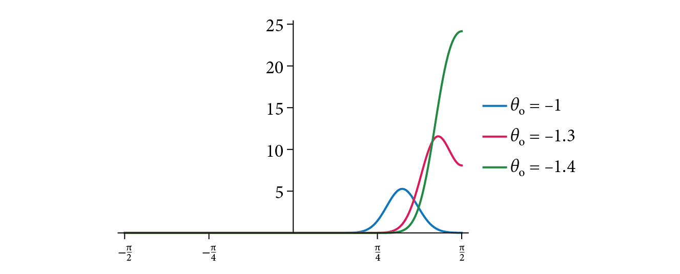
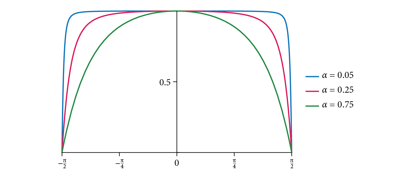
Figure 9.26 shows a plot of the Trowbridge–Reitz function for a few values of . Observe how the function is close to one over much of the domain but falls to zero at grazing angles, where masking becomes dominant. Increasing the surface roughness (i.e., higher values of ) causes the function to fall off more quickly.

9.6.3 The Masking-Shadowing Function

The BSDF is a function of two directional arguments, and each is subject to occlusion effects caused by the surface microstructure. For viewing and lighting directions, these are respectively denoted as masking and shadowing. To handle both cases, the masking function must be generalized into a masking-shadowing function that gives the fraction of microfacets in a differential area that are simultaneously visible from both directions and .

We know that gives the fraction of microfacets that are visible from the direction , and gives the fraction for . If we assume that masking and shadowing are statistically independent events, then these probabilities can simply be multiplied together:

However, this independence assumption is a rather severe approximation that tends to overestimate the amount of shadowing and masking. This can produce undesirable dark regions in rendered images.

We instead rely on an approximation that accounts for the property that a microfacet with a higher amount of elevation relative to the macrosurface is more likely to be observed from both and . If the heights of microfacets are normally distributed, a less conservative model for taking height-based correlation into account can be derived:

The bidirectional form of implements this equation based on the previously defined Lambda() function.

9.6.4 Sampling the Distribution of Visible Normals

Efficient rendering using microfacet theory hinges on our ability to determine the microfacet encountered by a particular incident ray—in essence, this operation must emulate the process of finding an intersection with the surface microstructure. Thanks to its stochastic definition, an actual ray tracing operation is fortunately not needed: the intersected microfacet follows a known statistical distribution that depends on the roughness and the direction of the incident ray.

Recall the normalization criterion from Equation (9.17), which stated that the set of visible microfacets (left hand side) occupy the same area as the underlying macrosurface (right hand side) when observed from given direction with elevation angle :

The probability of a ray interacting with a particular microfacet is directly proportional to its visible area; hence this equation can be seen to encapsulate the distribution that should be used. Following division of both sides by , the integral on the left hand side equals one—in other words, it turns into a normalized density that we shall refer to as the distribution of visible normals:

It describes the projected area of forward-facing normals, where the first term involving the masking function specifies an -dependent normalization factor. The method D() evaluates this density function.

Two upcoming microfacet BSDFs will rely on the ability to sample microfacet normals according to this density. At this point, one would ordinarily apply the inversion method (Section 2.3) to Equation (9.23) to build a sampling algorithm, but this leads to a relatively complex and approximate method: part of the problem is that the central inversion step lacks an analytic solution. We instead follow a simple geometric approach that exploits the definition of the microsurface in terms of an arrangement of many identical truncated spheres or ellipsoids.

Before implementing the sampling routine, we will quickly take care of the method that returns the associated PDF, which is simply another name for the D() method.

Figure 9.27 illustrates the high-level idea: it suffices to focus on a single ellipsoidal or spherical bump and perpendicularly project parallel rays from an incident direction onto its surface. The resulting normal directions will then be distributed according to the density function .

An observation illustrated in Figure 9.28 can be used to further simplify this task: by applying the inverse of the ellipsoid’s scaling transformation, the problem reduces to the simpler isotropic case. For this, we must transform the incident direction to the hemispherical configuration, perform a hemispherical sampling step, and then re-transform the resulting points back to the ellipsoidal state. The Sample_wm() method realizes this sequence of steps.

The first transformation to the hemispherical configuration is accomplished by applying the component-wise scaling factors and to the incident direction and renormalizing. By convention, microfacet normals point into the upper hemisphere, and we potentially flip the incident direction so that both directions are consistently oriented.

Next, we complete the unit vector to an orthonormal basis (T1, T2, wh). The particular construction below satisfies the additional constraint that T1 is perpendicular to the macroscopic normal .

Figure 9.29 illustrates the geometry of the projection. When is perpendicularly incident (first column), the hemisphere projects onto a disk. Non-perpendicular incidence (columns 2–4) reveals more interesting behavior: the bottom half that corresponds to the perpendicular projection of the tangential half-disk (blue) undergoes a scaling given by along the vertical axis (i.e., the T2 axis). Because the transformation is uniform, we can sample this set using a vertical affine transformation of uniform points on the disk.

Let denote a point on the unit disk. For a given , the -component lies on the interval , where specifies the maximum height. Due to non-perpendicular projection, this interval must now be reduced to , which requires an affine transformation with scale and offset . The following fragment efficiently performs this transformation using the Lerp() function.

The last step projects the computed position onto the hemisphere and computes its 3D coordinates. Finally, it reapplies the ellipsoidal transformation and returns the result.

Note that it may seem that we should divide instead of multiplying by and to realize the inverse of the transformation from the fragment <<Transform w to hemispherical configuration>>. This ostensible blunder is explained by the property that normals transform according to the inverse transpose of linear transformations (Section 3.10.3).

9.6.5 The Torrance–Sparrow Model

We can finally explain how the ConductorBxDF handles rough microstructures via a BRDF model due to Torrance and Sparrow (1967). Instead of directly deriving their approach from first principles, we will instead explain how this model is sampled in pbrt, and then reverse-engineer the implied BRDF.

Combined with the visible normal sampling approach, the sampling routine of this model consists of three physically intuitive steps:

1. Given a viewing ray from direction , a microfacet normal is sampled from the visible normal distribution . This step encapsulates the process of intersecting the viewing ray with the random microstructure.
2. Reflection from the sampled microfacet is modeled using the law of specular reflection and the Fresnel equations, which yields the incident direction and a reflection coefficient that attenuates the light carried by the path.
3. The scattered light is finally scaled by to account for the effect of masking by other microfacets.

Our goal will be to determine the BRDF that represents this sequence of steps. For this, we must first find the probability density of the sampled incident direction . Although visible normal sampling was involved, it is important to note that is not distributed according to the visible normal distribution—to find its density, we must consider the sequence of steps that were used to obtain from .

Taking stock of the available information, we know that the probability density of is given by , and that is obtained from and using the law of specular reflection—that is,

This reflection mapping also has an inverse: the normal responsible for a specific reflection can be determined via

which is known as the half-angle or half-direction transform, as it gives the unique direction vector that lies halfway between and .

The Half-Direction Transform

Transitioning between half- and incident directions is effectively a change of variables, and the Jacobian determinant of the associated mapping enables the conversion of probability densities between these two spaces. The determinant is simple to find in flatland, as shown in Figure 9.30(a). In the two-dimensional setting, the half-direction mapping simplifies to

A slight perturbation of the incident angle (shaded green region) while keeping fixed requires a corresponding change to the microfacet angle (shaded blue region) to ensure that the law of specular reflection continues to hold. However, this perturbation to is smaller—half as small, to be precise—which directly follows from Equation (9.26). Indeed, the derivative of Equation (9.26) yields for the 2D case.

The 3D case initially appears challenging due to the varied behavior shown in Figure 9.30(b–d). Fortunately, working with infinitesimal sets leads to a simple analytic expression that can be derived by expressing differential solid angles around and using spherical coordinates:

The expression can be simplified by noting that the law of specular reflection implies and in a spherical coordinate system oriented around :

The resulting Jacobian determinant can be thus conveniently expressed in terms of the microfacet normal and either or .

Torrance–Sparrow PDF

With the relationship of Equation (9.27) at hand, we are now able to evaluate the probability per unit solid angle of the sampled incident directions obtained through the combination of visible normal sampling and the reflection mapping:

where depends on via the half-direction transform in Equation (9.25). The following previously undefined fragment incorporates these observations into ConductorBxDF::PDF().

The sign-related differences between equation and implementation ensure correct operation when the incident ray lies below the surface.

Torrance–Sparrow BRDF

The sampling routine of any BRDF model encodes a local strategy for importance sampling the scattering equation, (4.14). Here, we are dealing with an opaque surface, so the integral is only over the hemisphere. The single-sample Monte Carlo estimator is then

where denotes the sample’s probability per unit solid angle.

Recall our earlier introduction of the Torrance–Sparrow sampling routine as a composition of physically intuitive steps: intersecting a ray against the random microstructure via visible normal sampling, computation of via the law of reflection, and attenuation of the incident radiance by the Fresnel and masking factors. The radiance computed in this way should agree with the Monte Carlo estimate from Equation (9.29), which means that must satisfy the identity

We will simply solve this equation to obtain . Further substituting the PDF of the Torrance–Sparrow model from Equation (9.28) yields the BRDF

Inserting the definition of the visible normal distribution from Equation (9.23) and assuming directions in the positive hemisphere results in the common form of the Torrance–Sparrow BRDF:

We will, however, make a small adjustment to the above expression: Section 9.6.3 introduced a more accurate bidirectional masking-shadowing factor that accounts for height correlations on the microstructure. We use it to replace the product of unidirectional factors:

One of the nice things about the Torrance–Sparrow model is that the derivation does not depend on the particular microfacet distribution being used. Furthermore, it does not depend on a particular Fresnel function and can be used for both conductors and dielectrics. However, the relationship between and used in the derivation does depend on the assumption of specular reflection from microfacets, and the refractive variant of this model will require suitable modifications.

Evaluating the terms of the Torrance–Sparrow BRDF is straightforward.

Incident and outgoing directions at glancing angles need to be handled explicitly to avoid the generation of NaN values:

Note that the Fresnel term is based on the angle of incidence relative to the microfacet (i.e., ) rather than the macrosurface.

Torrance–Sparrow Sampling

The sampling procedure follows the sequence of steps outlined at the beginning of this subsection. It first uses Sample_wm() to find a microfacet orientation and reflects the outgoing direction about the microfacet’s normal to find before evaluating the BRDF and density function.

A curious situation arises when the sampled microfacet normal leads to a computed direction that lies below the macroscopic surface. In a real microstructure, this would mean that light travels deeper into a crevice, to be scattered a second or third time. However, the presented ConductorBxDF only simulates a single interaction and thus marks such samples as invalid. This reveals one of the main flaws of the presented model: objects with significant roughness may appear too dark due to this lack of multiple scattering. Addressing issues related to energy loss is an active topic of research; see the “Further Reading” section for more information.

We omit the fragment <<Compute PDF of wi for microfacet reflection>> that follows ConductorBxDF::PDF().

Visible normal sampling is still a relatively new development: for several decades, microfacet models relied on sampling directly proportional to the microfacet distribution, which tends to produce noisier renderings since some terms of the BRDF are not sampled exactly. Figure 9.31 compares this classical approach to what is now implemented in pbrt.