A.5 Sampling Multidimensional Functions

Multidimensional sampling is also common in pbrt, most frequently when sampling points on the surfaces of shapes and sampling directions after scattering at points. This section therefore works through the derivations and implementations of algorithms for sampling in a number of useful multidimensional domains. Some of them involve separable PDFs where each dimension can be sampled independently, while others use the approach of sampling from marginal and conditional density functions that was introduced in Section 2.4.2.

A.5.1 Sampling a Unit Disk

Uniformly sampling a unit disk can be tricky because it has an incorrect intuitive solution. The wrong approach is the seemingly obvious one of sampling its polar coordinates uniformly: r equals xi 1 comma theta equals 2 pi xi 2 . Although the resulting point is both random and inside the disk, it is not uniformly distributed; it actually clumps samples near the center of the disk. Figure A.6(a) shows a plot of samples on the unit disk when this mapping was used for a set of uniform random samples left-parenthesis xi 1 comma xi 2 right-parenthesis . Figure A.6(b) shows uniformly distributed samples resulting from the following correct approach.

Figure A.6: (a) When the obvious but incorrect mapping of uniform random variables to points on the disk is used, the resulting distribution is not uniform and the samples are more likely to be near the center of the disk. (b) The correct mapping gives a uniform distribution of points.

Since we would like to sample uniformly with respect to area, the PDF p left-parenthesis x comma y right-parenthesis must be a constant. By the normalization constraint, p left-parenthesis x comma y right-parenthesis equals 1 slash pi . If we transform into polar coordinates, we have p left-parenthesis r comma theta right-parenthesis equals r slash pi given the relationship between probability densities in Cartesian coordinates and polar coordinates that was derived in Section 2.4.1, Equation (2.22).

We can now compute the marginal and conditional densities:

StartLayout 1st Row 1st Column p left-parenthesis r right-parenthesis 2nd Column equals integral Subscript 0 Superscript 2 pi Baseline p left-parenthesis r comma theta right-parenthesis normal d theta Subscript Baseline equals 2 r 2nd Row 1st Column p left-parenthesis theta vertical-bar r right-parenthesis 2nd Column equals StartFraction p left-parenthesis r comma theta right-parenthesis Over p left-parenthesis r right-parenthesis EndFraction equals StartFraction 1 Over 2 pi EndFraction period EndLayout

The fact that p left-parenthesis theta vertical-bar r right-parenthesis is a constant should make sense because of the symmetry of the disk. Integrating and inverting to find upper P left-parenthesis r right-parenthesis , upper P Superscript negative 1 Baseline left-parenthesis r right-parenthesis , upper P left-parenthesis theta right-parenthesis , and upper P Superscript negative 1 Baseline left-parenthesis theta right-parenthesis , we can find that the correct solution to generate uniformly distributed samples on a disk is

StartLayout 1st Row 1st Column r 2nd Column equals StartRoot xi 1 EndRoot 2nd Row 1st Column theta 2nd Column equals 2 pi xi 2 period EndLayout

Taking the square root of xi 1 effectively pushes the samples back toward the edge of the disk, counteracting the clumping referred to earlier.

<<Sampling Inline Functions>>+=  
Point2f SampleUniformDiskPolar(Point2f u) { Float r = std::sqrt(u[0]); Float theta = 2 * Pi * u[1]; return {r * std::cos(theta), r * std::sin(theta)}; }

The inversion method, InvertUniformDiskPolarSample(), is straightforward and is not included here.

Although this mapping solves the problem at hand, it distorts areas on the disk; areas on the unit square are elongated or compressed when mapped to the disk (Figure A.7). This distortion can reduce the effectiveness of stratified sampling patterns by making the strata less compact. A better approach that avoids this problem is a “concentric” mapping from the unit square to the unit disk. The concentric mapping takes points in the square left-bracket negative 1 comma 1 right-bracket squared to the unit disk by uniformly mapping concentric squares to concentric circles (Figure A.8).

Figure A.7: The mapping from 2D random samples to points on the disk implemented in SampleUniformDiskPolar() distorts areas substantially. Each section of the disk here has equal area and represents one-eighth of the unit square of uniform random samples in each direction. In general, we would prefer a mapping that did a better job at mapping nearby left-parenthesis xi 1 comma xi 2 right-parenthesis values to nearby points on the disk.

Figure A.8: The concentric mapping maps squares to circles, giving a less distorted mapping than the first method shown for uniformly sampling points on the unit disk. It is based on mapping triangular wedges of the unit square to pie-shaped wedges of the disk, as shown here.

The mapping turns wedges of the square into slices of the disk. For example, points in the shaded area in Figure A.8 are mapped to left-parenthesis r comma theta right-parenthesis  by

StartLayout 1st Row 1st Column r 2nd Column equals x 2nd Row 1st Column theta 2nd Column equals StartFraction y Over x EndFraction StartFraction pi Over 4 EndFraction period EndLayout

See Figure A.9. The other seven wedges are handled analogously.

Figure A.9: Triangular wedges of the square are mapped into left-parenthesis r comma theta right-parenthesis pairs in pie-shaped slices of the disk in the SampleUniformDiskConcentric() function.

<<Sampling Inline Functions>>+=  
Point2f SampleUniformDiskConcentric(Point2f u) { <<Map u to left-bracket negative 1 comma 1 right-bracket squared and handle degeneracy at the origin>> 
Point2f uOffset = 2 * u - Vector2f(1, 1); if (uOffset.x == 0 && uOffset.y == 0) return {0, 0};
<<Apply concentric mapping to point>> 
Float theta, r; if (std::abs(uOffset.x) > std::abs(uOffset.y)) { r = uOffset.x; theta = PiOver4 * (uOffset.y / uOffset.x); } else { r = uOffset.y; theta = PiOver2 - PiOver4 * (uOffset.x / uOffset.y); } return r * Point2f(std::cos(theta), std::sin(theta));
}

For the following, the random samples are mapped to the left-bracket negative 1 comma 1 right-bracket squared square. The left-parenthesis 0 comma 0 right-parenthesis point is then handled specially so that the following code does not need to avoid dividing by zero.

<<Map u to left-bracket negative 1 comma 1 right-bracket squared and handle degeneracy at the origin>>= 
Point2f uOffset = 2 * u - Vector2f(1, 1); if (uOffset.x == 0 && uOffset.y == 0) return {0, 0};

All the other points are transformed using the mapping from square wedges to disk slices by way of computing left-parenthesis r comma theta right-parenthesis polar coordinates for them. The following implementation is carefully crafted so that the mapping is continuous across adjacent slices.

<<Apply concentric mapping to point>>= 
Float theta, r; if (std::abs(uOffset.x) > std::abs(uOffset.y)) { r = uOffset.x; theta = PiOver4 * (uOffset.y / uOffset.x); } else { r = uOffset.y; theta = PiOver2 - PiOver4 * (uOffset.x / uOffset.y); } return r * Point2f(std::cos(theta), std::sin(theta));

The corresponding inversion function, InvertUniformDiskConcentricSample(), is not included in the text here.

A.5.2 Uniformly Sampling Hemispheres and Spheres

The area of a unit hemisphere is 2 pi , and thus the PDF for uniform sampling must be p left-parenthesis omega right-parenthesis equals 1 slash left-parenthesis 2 pi right-parenthesis .

We will use spherical coordinates to derive a sampling algorithm. Using Equation (2.23) from Section 2.4.1, we have p left-parenthesis theta comma phi right-parenthesis equals sine theta slash left-parenthesis 2 pi right-parenthesis . This density function is separable. Because phi ranges from 0 to 2 pi and must have a constant PDF, p left-parenthesis phi right-parenthesis equals 1 slash left-parenthesis 2 pi right-parenthesis and therefore p left-parenthesis theta right-parenthesis equals sine theta . The two CDFs follow:

StartLayout 1st Row 1st Column upper P left-parenthesis theta right-parenthesis 2nd Column equals integral Subscript 0 Superscript theta Baseline sine theta prime normal d theta Subscript Superscript prime Baseline equals 1 minus cosine theta 2nd Row 1st Column upper P left-parenthesis phi right-parenthesis 2nd Column equals integral Subscript 0 Superscript phi Baseline StartFraction 1 Over 2 pi EndFraction normal d phi Superscript prime Baseline equals StartFraction phi Over 2 pi EndFraction period EndLayout

Inverting these functions is straightforward, and in this case we can tidy the result by replacing 1 minus xi Subscript with xi Subscript , giving

StartLayout 1st Row 1st Column theta 2nd Column equals cosine Superscript negative 1 Baseline xi 1 2nd Row 1st Column phi 2nd Column equals 2 pi xi 2 period EndLayout

Converting back to Cartesian coordinates, we get the final sampling formulae:

StartLayout 1st Row 1st Column x 2nd Column equals sine theta cosine phi equals cosine left-parenthesis 2 pi xi 2 right-parenthesis StartRoot 1 minus xi 1 squared EndRoot 2nd Row 1st Column y 2nd Column equals sine theta sine phi equals sine left-parenthesis 2 pi xi 2 right-parenthesis StartRoot 1 minus xi 1 squared EndRoot 3rd Row 1st Column z 2nd Column equals cosine theta equals xi 1 period EndLayout

This sampling strategy is implemented in the following code. Two uniform random numbers are provided in u, and a vector on the hemisphere is returned.

<<Sampling Inline Functions>>+=  
Vector3f SampleUniformHemisphere(Point2f u) { Float z = u[0]; Float r = SafeSqrt(1 - Sqr(z)); Float phi = 2 * Pi * u[1]; return {r * std::cos(phi), r * std::sin(phi), z}; }

For each PDF evaluation function, it is important to be clear which PDF is being evaluated—for example, we have already seen directional probabilities expressed both in terms of solid angle and in terms of left-parenthesis theta comma phi right-parenthesis . For hemispheres (and all other directional sampling in pbrt), these functions return probability with respect to solid angle. Thus, the uniform hemisphere PDF function is trivial and does not require that the direction be passed to it.

<<Sampling Inline Functions>>+=  
Float UniformHemispherePDF() { return Inv2Pi; }

The inverse sampling method can be derived starting from Equation (A.17).

<<Sampling Inline Functions>>+=  
Point2f InvertUniformHemisphereSample(Vector3f w) { Float phi = std::atan2(w.y, w.x); if (phi < 0) phi += 2 * Pi; return Point2f(w.z, phi / (2 * Pi)); }

Sampling the full sphere uniformly over its area follows almost exactly the same derivation, which we omit here. The end result is

StartLayout 1st Row 1st Column x 2nd Column equals cosine left-parenthesis 2 pi xi 2 right-parenthesis StartRoot 1 minus z squared EndRoot equals cosine left-parenthesis 2 pi xi 2 right-parenthesis 2 StartRoot xi 1 left-parenthesis 1 minus xi 1 right-parenthesis EndRoot 2nd Row 1st Column y 2nd Column equals sine left-parenthesis 2 pi xi 2 right-parenthesis StartRoot 1 minus z squared EndRoot equals sine left-parenthesis 2 pi xi 2 right-parenthesis 2 StartRoot xi 1 left-parenthesis 1 minus xi 1 right-parenthesis EndRoot 3rd Row 1st Column z 2nd Column equals 1 minus 2 xi 1 period EndLayout

<<Sampling Inline Functions>>+=  
Vector3f SampleUniformSphere(Point2f u) { Float z = 1 - 2 * u[0]; Float r = SafeSqrt(1 - Sqr(z)); Float phi = 2 * Pi * u[1]; return {r * std::cos(phi), r * std::sin(phi), z}; }

The PDF is 1 slash left-parenthesis 4 pi right-parenthesis , one over the surface area of the unit sphere.

<<Sampling Inline Functions>>+=  
Float UniformSpherePDF() { return Inv4Pi; }

The sampling inversion method also follows directly.

<<Sampling Inline Functions>>+=  
Point2f InvertUniformSphereSample(Vector3f w) { Float phi = std::atan2(w.y, w.x); if (phi < 0) phi += 2 * Pi; return Point2f((1 - w.z) / 2, phi / (2 * Pi)); }

A.5.3 Cosine-Weighted Hemisphere Sampling

As we saw in the discussion of importance sampling (Section 2.2.2), it is often useful to sample from a distribution that has a shape similar to that of the integrand being estimated. Many light transport integrals include a cosine factor, and therefore it is useful to have a method that generates directions according to a cosine-weighted distribution on the hemisphere. Such a method gives samples that are more likely to be close to the top of the hemisphere, where the cosine term has a large value, rather than near the bottom, where the cosine term is small.

Mathematically, this means that we would like to sample directions omega Subscript from a PDF

p left-parenthesis omega right-parenthesis proportional-to cosine theta period

Normalizing as usual,

StartLayout 1st Row 1st Column integral Underscript script upper H squared Endscripts p left-parenthesis omega Subscript Baseline right-parenthesis normal d omega Subscript 2nd Column equals 1 2nd Row 1st Column integral Subscript 0 Superscript 2 pi Baseline integral Subscript 0 Superscript StartFraction pi Over 2 EndFraction Baseline c cosine theta sine theta normal d theta Subscript Baseline normal d phi Subscript 2nd Column equals 1 3rd Row 1st Column c Baseline 2 pi integral Subscript 0 Superscript pi slash 2 Baseline cosine theta sine theta normal d theta Subscript 2nd Column equals 1 4th Row 1st Column c 2nd Column equals StartFraction 1 Over pi EndFraction period EndLayout

Thus,

p left-parenthesis theta comma phi right-parenthesis equals StartFraction 1 Over pi EndFraction cosine theta sine theta period

We could compute the marginal and conditional densities as before, but instead we can use a technique known as Malley’s method to generate these cosine-weighted points. The idea behind Malley’s method is that if we choose points uniformly from the unit disk and then generate directions by projecting the points on the disk up to the hemisphere above it, the result will have a cosine-weighted distribution of directions (Figure A.10).

Figure A.10: Malley’s Method. To sample direction vectors from a cosine-weighted distribution, uniformly sample points on the unit disk and project them up to the unit hemisphere.

Why does this work? Let left-parenthesis r comma phi right-parenthesis be the polar coordinates of the point chosen on the disk (note that we are using phi instead of the usual theta for the polar angle here). From Section A.5.1, we know that the joint density p left-parenthesis r comma phi right-parenthesis equals r slash pi gives the density of a point sampled on the disk.

Now, we map this point to the hemisphere. The vertical projection gives sine theta equals r , which is easily seen from Figure A.10. To complete the left-parenthesis r comma phi right-parenthesis equals left-parenthesis sine theta comma phi right-parenthesis right-arrow left-parenthesis theta comma phi right-parenthesis transformation, we need the determinant of the Jacobian

StartAbsoluteValue upper J Subscript upper T Baseline EndAbsoluteValue equals Start 2 By 2 Determinant 1st Row 1st Column cosine theta 2nd Column 0 2nd Row 1st Column 0 2nd Column 1 EndDeterminant equals cosine theta period

Therefore,

p left-parenthesis theta comma phi right-parenthesis equals StartAbsoluteValue upper J Subscript upper T Baseline EndAbsoluteValue p left-parenthesis r comma phi right-parenthesis equals cosine theta StartFraction r Over pi EndFraction equals StartFraction cosine theta sine theta Over pi EndFraction comma

which is exactly what we wanted! We have used the transformation method to prove that Malley’s method generates directions with a cosine-weighted distribution. Note that this technique works with any uniform disk sampling approach, so we can use the earlier concentric mapping just as well as the simpler left-parenthesis r comma theta right-parenthesis equals left-parenthesis StartRoot xi 1 EndRoot comma 2 pi xi 2 right-parenthesis method.

<<Sampling Inline Functions>>+=  
Vector3f SampleCosineHemisphere(Point2f u) { Point2f d = SampleUniformDiskConcentric(u); Float z = SafeSqrt(1 - Sqr(d.x) - Sqr(d.y)); return Vector3f(d.x, d.y, z); }

Because directional PDFs in pbrt are defined with respect to solid angle, the PDF function returns the value cosine theta slash pi .

<<Sampling Inline Functions>>+=  
Float CosineHemispherePDF(Float cosTheta) { return cosTheta * InvPi; }

Finally, a directional sample can be inverted purely from its left-parenthesis x comma y right-parenthesis coordinates on the disk.

<<Sampling Inline Functions>>+=  
Point2f InvertCosineHemisphereSample(Vector3f w) { return InvertUniformDiskConcentricSample({w.x, w.y}); }

A.5.4 Sampling Within a Cone

It is sometimes useful to be able to uniformly sample rays in a cone of directions. This distribution is separable in left-parenthesis theta comma phi right-parenthesis , with p left-parenthesis phi right-parenthesis equals 1 slash left-parenthesis 2 pi right-parenthesis , and so we therefore need to derive a method to sample a direction theta up to the maximum angle of the cone, theta Subscript normal m normal a normal x . Incorporating the sine theta term from the measure on the unit sphere from Equation (4.8), we have

StartLayout 1st Row 1st Column 1 2nd Column equals c integral Subscript 0 Superscript theta Subscript normal m normal a normal x Baseline Baseline sine theta normal d theta Subscript Baseline 2nd Row 1st Column Blank 2nd Column equals c left-parenthesis 1 minus cosine theta Subscript normal m normal a normal x Baseline right-parenthesis period EndLayout

So p left-parenthesis theta right-parenthesis equals sine theta slash left-parenthesis 1 minus cosine theta Subscript normal m normal a normal x Baseline right-parenthesis and p left-parenthesis omega right-parenthesis equals 1 slash left-parenthesis 2 pi left-parenthesis 1 minus cosine theta Subscript normal m normal a normal x Baseline right-parenthesis right-parenthesis .

<<Sampling Inline Functions>>+=  
Float UniformConePDF(Float cosThetaMax) { return 1 / (2 * Pi * (1 - cosThetaMax)); }

The PDF can be integrated to find the CDF and the sampling technique for theta follows:

cosine theta equals left-parenthesis 1 minus xi Subscript Baseline right-parenthesis plus xi Subscript Baseline cosine theta Subscript normal m normal a normal x Baseline period

The following code samples a canonical cone around the left-parenthesis 0 comma 0 comma 1 right-parenthesis axis; the sample can be transformed to cones with other orientations using the Frame class.

<<Sampling Inline Functions>>+= 
Vector3f SampleUniformCone(Point2f u, Float cosThetaMax) { Float cosTheta = (1 - u[0]) + u[0] * cosThetaMax; Float sinTheta = SafeSqrt(1 - Sqr(cosTheta)); Float phi = u[1] * 2 * Pi; return SphericalDirection(sinTheta, cosTheta, phi); }

The inversion function, InvertUniformConeSample(), is not included here.

A.5.5 Piecewise-Constant 2D Distributions

Building on the approach for sampling piecewise-constant 1D distributions in Section A.4.7, we can apply the marginal-conditional approach to sample from piecewise-constant 2D distributions. We will consider the case of a 2D function defined over a user-specified domain by a 2D array of n Subscript u Baseline times n Subscript v sample values. This case is particularly useful for generating samples from distributions defined by image maps and environment maps.

Consider a 2D function f left-parenthesis u comma v right-parenthesis defined by a set of n Subscript u Baseline times n Subscript v values f left-bracket u Subscript i Baseline comma v Subscript j Baseline right-bracket where u Subscript i Baseline element-of left-bracket 0 comma 1 comma ellipsis comma n Subscript u Baseline minus 1 right-bracket , v Subscript j Baseline element-of left-bracket 0 comma 1 comma ellipsis comma n Subscript v Baseline minus 1 right-bracket , and f left-bracket u Subscript i Baseline comma v Subscript j Baseline right-bracket gives the constant value of f over the range left-bracket i slash n Subscript u Baseline comma left-parenthesis i plus 1 right-parenthesis slash n Subscript u Baseline right-parenthesis times left-bracket j slash n Subscript v Baseline comma left-parenthesis j plus 1 right-parenthesis slash n Subscript v Baseline right-parenthesis . Given continuous values left-parenthesis u comma v right-parenthesis , we will use left-parenthesis u overTilde comma v overTilde right-parenthesis to denote the corresponding discrete left-parenthesis u Subscript i Baseline comma v Subscript j Baseline right-parenthesis indices, with u overTilde equals left floor n Subscript u Baseline u right floor and v overTilde equals left floor n Subscript v Baseline v right floor so that f left-parenthesis u comma v right-parenthesis equals f left-bracket u overTilde comma v overTilde right-bracket .

Integrals of f are sums of f left-bracket u Subscript i Baseline comma v Subscript j Baseline right-bracket , so that, for example, the integral of f over the domain is

upper I Subscript f Baseline equals integral integral f left-parenthesis u comma v right-parenthesis normal d u normal d v equals StartFraction 1 Over n Subscript u Baseline n Subscript v Baseline EndFraction sigma-summation Underscript i equals 0 Overscript n Subscript u Baseline minus 1 Endscripts sigma-summation Underscript j equals 0 Overscript n Subscript v Baseline minus 1 Endscripts f left-bracket u Subscript i Baseline comma v Subscript j Baseline right-bracket period

Using the definition of the PDF and the integral of f , we can find f ’s PDF,

p left-parenthesis u comma v right-parenthesis equals StartFraction f left-parenthesis u comma v right-parenthesis Over integral integral f left-parenthesis u comma v right-parenthesis normal d u normal d v EndFraction equals StartFraction f left-bracket u overTilde comma v overTilde right-bracket Over 1 slash left-parenthesis n Subscript u Baseline n Subscript v Baseline right-parenthesis sigma-summation Underscript i equals 0 Overscript n Subscript u Baseline minus 1 Endscripts sigma-summation Underscript j equals 0 Overscript n Subscript v Baseline minus 1 Endscripts f left-bracket u Subscript i Baseline comma v Subscript j Baseline right-bracket EndFraction period

Recalling Equation (2.24), the marginal density p left-parenthesis v right-parenthesis can be computed as a sum of f left-bracket u Subscript i Baseline comma v Subscript j Baseline right-bracket values

p left-parenthesis v right-parenthesis equals integral p left-parenthesis u comma v right-parenthesis normal d u equals StartFraction left-parenthesis 1 slash n Subscript u Baseline right-parenthesis sigma-summation Underscript i equals 0 Overscript n Subscript u Baseline minus 1 Endscripts f left-bracket u Subscript i Baseline comma v overTilde right-bracket Over upper I Subscript f Baseline EndFraction period

Because this function only depends on v overTilde , it is thus itself a piecewise-constant 1D function, p left-bracket v overTilde right-bracket , defined by n Subscript v values. The 1D sampling machinery from Section A.4.7 can be applied to sampling from its distribution.

Given a v sample, the conditional density p left-parenthesis u vertical-bar v right-parenthesis is then

p left-parenthesis u vertical-bar v right-parenthesis equals StartFraction p left-parenthesis u comma v right-parenthesis Over p left-parenthesis v right-parenthesis EndFraction equals StartFraction f left-bracket u overTilde comma v overTilde right-bracket slash upper I Subscript f Baseline Over p left-bracket v overTilde right-bracket EndFraction period

Note that, given a particular value of v overTilde , p left-bracket u overTilde vertical-bar v overTilde right-bracket is a piecewise-constant 1D function of u overTilde that can be sampled with the usual 1D approach. There are n Subscript v such distinct 1D conditional densities, one for each possible value of v overTilde .

Putting this all together, the PiecewiseConstant2D class provides functionality similar to PiecewiseConstant1D, except that it generates samples from piecewise-constant 2D distributions.

<<PiecewiseConstant2D Definition>>= 
class PiecewiseConstant2D { public: <<PiecewiseConstant2D Public Methods>> 
PiecewiseConstant2D() = default; PiecewiseConstant2D(Allocator alloc) : pConditionalV(alloc), pMarginal(alloc) {} PiecewiseConstant2D(pstd::span<const Float> data, int nx, int ny, Allocator alloc = {}) : PiecewiseConstant2D(data, nx, ny, Bounds2f(Point2f(0, 0), Point2f(1, 1)), alloc) {} explicit PiecewiseConstant2D(const Array2D<Float> &data, Allocator alloc = {}) : PiecewiseConstant2D(pstd::span<const Float>(data), data.XSize(), data.YSize(), alloc) {} PiecewiseConstant2D(const Array2D<Float> &data, Bounds2f domain, Allocator alloc = {}) : PiecewiseConstant2D(pstd::span<const Float>(data), data.XSize(), data.YSize(), domain, alloc) {} PBRT_CPU_GPU size_t BytesUsed() const { return pConditionalV.size() * (pConditionalV[0].BytesUsed() + sizeof(pConditionalV[0])) + pMarginal.BytesUsed(); } PBRT_CPU_GPU Bounds2f Domain() const { return domain; } PBRT_CPU_GPU Point2i Resolution() const { return {int(pConditionalV[0].size()), int(pMarginal.size())}; } std::string ToString() const { return StringPrintf("[ PiecewiseConstant2D domain: %s pConditionalV: %s " "pMarginal: %s ]", domain, pConditionalV, pMarginal); } static void TestCompareDistributions(const PiecewiseConstant2D &da, const PiecewiseConstant2D &db, Float eps = 1e-5); PiecewiseConstant2D(pstd::span<const Float> func, int nu, int nv, Bounds2f domain, Allocator alloc = {}) : domain(domain), pConditionalV(alloc), pMarginal(alloc) { for (int v = 0; v < nv; ++v) <<Compute conditional sampling distribution for v overTilde >> 
pConditionalV.emplace_back(func.subspan(v * nu, nu), domain.pMin[0], domain.pMax[0], alloc);
<<Compute marginal sampling distribution p left-bracket v overTilde right-bracket >> 
pstd::vector<Float> marginalFunc; for (int v = 0; v < nv; ++v) marginalFunc.push_back(pConditionalV[v].Integral()); pMarginal = PiecewiseConstant1D(marginalFunc, domain.pMin[1], domain.pMax[1], alloc);
} Float Integral() const { return pMarginal.Integral(); } Point2f Sample(Point2f u, Float *pdf = nullptr, Point2i *offset = nullptr) const { Float pdfs[2]; Point2i uv; Float d1 = pMarginal.Sample(u[1], &pdfs[1], &uv[1]); Float d0 = pConditionalV[uv[1]].Sample(u[0], &pdfs[0], &uv[0]); if (pdf) *pdf = pdfs[0] * pdfs[1]; if (offset) *offset = uv; return Point2f(d0, d1); } Float PDF(Point2f pr) const { Point2f p = Point2f(domain.Offset(pr)); int iu = Clamp(int(p[0] * pConditionalV[0].size()), 0, pConditionalV[0].size() - 1); int iv = Clamp(int(p[1] * pMarginal.size()), 0, pMarginal.size() - 1); return pConditionalV[iv].func[iu] / pMarginal.Integral(); } pstd::optional<Point2f> Invert(Point2f p) const { pstd::optional<Float> mInv = pMarginal.Invert(p[1]); if (!mInv) return {}; Float p1o = (p[1] - domain.pMin[1]) / (domain.pMax[1] - domain.pMin[1]); if (p1o < 0 || p1o > 1) return {}; int offset = Clamp(p1o * pConditionalV.size(), 0, pConditionalV.size() - 1); pstd::optional<Float> cInv = pConditionalV[offset].Invert(p[0]); if (!cInv) return {}; return Point2f(*cInv, *mInv); }
private: <<PiecewiseConstant2D Private Members>> 
Bounds2f domain; pstd::vector<PiecewiseConstant1D> pConditionalV; PiecewiseConstant1D pMarginal;
};

Its constructor has two tasks. First, it computes a 1D conditional sampling density p left-bracket u overTilde vertical-bar v overTilde right-bracket for each of the n Subscript v individual v overTilde values using Equation (A.17). It then computes the marginal sampling density p left-bracket v overTilde right-bracket with Equation (A.17). (PiecewiseConstant2D provides a variety of additional constructors, not included here, including ones that take an Array2D to specify the values. See the pbrt source code for details.)

<<PiecewiseConstant2D Public Methods>>= 
PiecewiseConstant2D(pstd::span<const Float> func, int nu, int nv, Bounds2f domain, Allocator alloc = {}) : domain(domain), pConditionalV(alloc), pMarginal(alloc) { for (int v = 0; v < nv; ++v) <<Compute conditional sampling distribution for v overTilde >> 
pConditionalV.emplace_back(func.subspan(v * nu, nu), domain.pMin[0], domain.pMax[0], alloc);
<<Compute marginal sampling distribution p left-bracket v overTilde right-bracket >> 
pstd::vector<Float> marginalFunc; for (int v = 0; v < nv; ++v) marginalFunc.push_back(pConditionalV[v].Integral()); pMarginal = PiecewiseConstant1D(marginalFunc, domain.pMin[1], domain.pMax[1], alloc);
}

<<PiecewiseConstant2D Private Members>>= 
Bounds2f domain;

PiecewiseConstant1D can directly compute the p left-bracket u overTilde vertical-bar v overTilde right-bracket distributions from each of the n Subscript v rows of n Subscript u function values, since they are laid out linearly in memory. The upper I Subscript f and p left-bracket v overTilde right-bracket terms from Equation (A.17) do not need to be included in the values passed to PiecewiseConstant1D since they have the same value for all the n Subscript u values and are thus just a constant scale that does not affect the normalized distribution that PiecewiseConstant1D computes.

<<Compute conditional sampling distribution for v overTilde >>= 
pConditionalV.emplace_back(func.subspan(v * nu, nu), domain.pMin[0], domain.pMax[0], alloc);

<<PiecewiseConstant2D Private Members>>+=  
pstd::vector<PiecewiseConstant1D> pConditionalV;

Given the conditional densities for each v overTilde value, we can find the 1D marginal density for sampling each one, p left-bracket v overTilde right-bracket . Because the PiecewiseConstant1D class has a method that provides the integral of its function, it is just necessary to copy these values to the marginalFunc buffer so they are stored linearly in memory for the PiecewiseConstant1D constructor.

<<Compute marginal sampling distribution p left-bracket v overTilde right-bracket >>= 
pstd::vector<Float> marginalFunc; for (int v = 0; v < nv; ++v) marginalFunc.push_back(pConditionalV[v].Integral()); pMarginal = PiecewiseConstant1D(marginalFunc, domain.pMin[1], domain.pMax[1], alloc);

<<PiecewiseConstant2D Private Members>>+= 
PiecewiseConstant1D pMarginal;

The integral of the function over the left-bracket 0 comma 1 right-bracket squared domain is made available via the Integral() method. Because the marginal distribution is the integral of one dimension, its integral gives the function’s full integral.

<<PiecewiseConstant2D Public Methods>>+=  
Float Integral() const { return pMarginal.Integral(); }

As described previously, in order to sample from the 2D distribution, first a sample is drawn from the p left-bracket v overTilde right-bracket marginal distribution in order to find the v coordinate of the sample. The offset of the sampled function value gives the integer v overTilde value that determines which of the precomputed conditional distributions should be used for sampling the u value. Figure A.11 illustrates this idea using a low-resolution image as an example.

Figure A.11: The Piecewise-Constant Sampling Distribution for a High-Dynamic-Range Environment Map. (a) The original environment map. (b) A low-resolution version of the marginal density function p left-bracket ModifyingAbove v With caret right-bracket and the conditional distributions for rows of the image. First the marginal 1D distribution is used to select a v value, giving a row of the image to sample. Rows with bright pixels are more likely to be sampled. Then, given a row, a value u is sampled from that row’s 1D distribution.

<<PiecewiseConstant2D Public Methods>>+=  
Point2f Sample(Point2f u, Float *pdf = nullptr, Point2i *offset = nullptr) const { Float pdfs[2]; Point2i uv; Float d1 = pMarginal.Sample(u[1], &pdfs[1], &uv[1]); Float d0 = pConditionalV[uv[1]].Sample(u[0], &pdfs[0], &uv[0]); if (pdf) *pdf = pdfs[0] * pdfs[1]; if (offset) *offset = uv; return Point2f(d0, d1); }

The value of the PDF for a given sample value is computed as the product of the conditional and marginal PDFs for sampling it.

<<PiecewiseConstant2D Public Methods>>+= 
Float PDF(Point2f pr) const { Point2f p = Point2f(domain.Offset(pr)); int iu = Clamp(int(p[0] * pConditionalV[0].size()), 0, pConditionalV[0].size() - 1); int iv = Clamp(int(p[1] * pMarginal.size()), 0, pMarginal.size() - 1); return pConditionalV[iv].func[iu] / pMarginal.Integral(); }

The Invert() method, not included here, inverts the provided sample by inverting the v sample using the marginal distribution and then inverting u via the appropriate conditional distribution.

A.5.6 Windowed Piecewise-Constant 2D Distributions

WindowedPiecewiseConstant2D generalizes the PiecewiseConstant2D class to allow the caller to specify a window that limits the sampling domain to a given rectangular subset of it. (This capability was key for the implementation of the PortalImageInfiniteLight in Section 12.5.3.) Before going into its implementation, we will start with the SummedAreaTable class, which provides some capabilities that make it easier to implement. We have encapsulated them in a stand-alone class, as they can be useful in other settings as well.

In 2D, a summed-area table is a 2D array where each element left-parenthesis x comma y right-parenthesis stores a sum of values from another array a :

s left-parenthesis x comma y right-parenthesis equals sigma-summation Underscript x prime equals 0 Overscript x minus 1 Endscripts sigma-summation Underscript y prime equals 0 Overscript y minus 1 Endscripts a left-parenthesis x prime comma y Superscript prime Baseline right-parenthesis comma

where here we have used C++’s zero-based array indexing convention.

Summed-area tables can be used to compute the sum of array values over rectangular regions of the original array in constant time. If the array a is interpreted as samples of a function, a summed-area table can efficiently compute integrals over arbitrary rectangular regions in a similar fashion. (Summed-area tables are therefore sometimes referred to as integral images.) They have a straightforward generalization to higher dimensions, though two of them suffice for pbrt’s needs.

<<SummedAreaTable Definition>>= 
class SummedAreaTable { public: <<SummedAreaTable Public Methods>> 
SummedAreaTable(const Array2D<Float> &values, Allocator alloc = {}) : sum(values.XSize(), values.YSize(), alloc) { sum(0, 0) = values(0, 0); <<Compute sums along first row and column>> 
for (int x = 1; x < sum.XSize(); ++x) sum(x, 0) = values(x, 0) + sum(x - 1, 0); for (int y = 1; y < sum.YSize(); ++y) sum(0, y) = values(0, y) + sum(0, y - 1);
<<Compute sums for the remainder of the entries>> 
for (int y = 1; y < sum.YSize(); ++y) for (int x = 1; x < sum.XSize(); ++x) sum(x, y) = (values(x, y) + sum(x - 1, y) + sum(x, y - 1) - sum(x - 1, y - 1));
} Float Integral(Bounds2f extent) const { double s = (((double)Lookup(extent.pMax.x, extent.pMax.y) - (double)Lookup(extent.pMin.x, extent.pMax.y)) + ((double)Lookup(extent.pMin.x, extent.pMin.y) - (double)Lookup(extent.pMax.x, extent.pMin.y))); return std::max<Float>(s / (sum.XSize() * sum.YSize()), 0); } std::string ToString() const;
private: <<SummedAreaTable Private Methods>> 
Float Lookup(Float x, Float y) const { <<Rescale left-parenthesis x comma y right-parenthesis to table resolution and compute integer coordinates>> 
x *= sum.XSize(); y *= sum.YSize(); int x0 = (int)x, y0 = (int)y;
<<Bilinearly interpolate between surrounding table values>> 
Float v00 = LookupInt(x0, y0), v10 = LookupInt(x0 + 1, y0); Float v01 = LookupInt(x0, y0 + 1), v11 = LookupInt(x0 + 1, y0 + 1); Float dx = x - int(x), dy = y - int(y); return (1 - dx) * (1 - dy) * v00 + (1 - dx) * dy * v01 + dx * (1 - dy) * v10 + dx * dy * v11;
} Float LookupInt(int x, int y) const { <<Return zero at lower boundaries>> 
if (x == 0 || y == 0) return 0;
<<Reindex left-parenthesis x comma y right-parenthesis and return actual stored value>> 
x = std::min(x - 1, sum.XSize() - 1); y = std::min(y - 1, sum.YSize() - 1); return sum(x, y);
}
<<SummedAreaTable Private Members>> 
Array2D<double> sum;
};

The constructor takes a 2D array of values that are used to initialize its sum array, which holds the corresponding sums. The first entry is easy: it is just the left-parenthesis 0 comma 0 right-parenthesis entry from the provided values array.

<<SummedAreaTable Public Methods>>= 
SummedAreaTable(const Array2D<Float> &values, Allocator alloc = {}) : sum(values.XSize(), values.YSize(), alloc) { sum(0, 0) = values(0, 0); <<Compute sums along first row and column>> 
for (int x = 1; x < sum.XSize(); ++x) sum(x, 0) = values(x, 0) + sum(x - 1, 0); for (int y = 1; y < sum.YSize(); ++y) sum(0, y) = values(0, y) + sum(0, y - 1);
<<Compute sums for the remainder of the entries>> 
for (int y = 1; y < sum.YSize(); ++y) for (int x = 1; x < sum.XSize(); ++x) sum(x, y) = (values(x, y) + sum(x - 1, y) + sum(x, y - 1) - sum(x - 1, y - 1));
}

<<SummedAreaTable Private Members>>= 
Array2D<double> sum;

All the remaining entries in sum can be computed incrementally. It is easiest to start out by computing sums as x varies with y equals 0 and vice versa.

<<Compute sums along first row and column>>= 
for (int x = 1; x < sum.XSize(); ++x) sum(x, 0) = values(x, 0) + sum(x - 1, 0); for (int y = 1; y < sum.YSize(); ++y) sum(0, y) = values(0, y) + sum(0, y - 1);

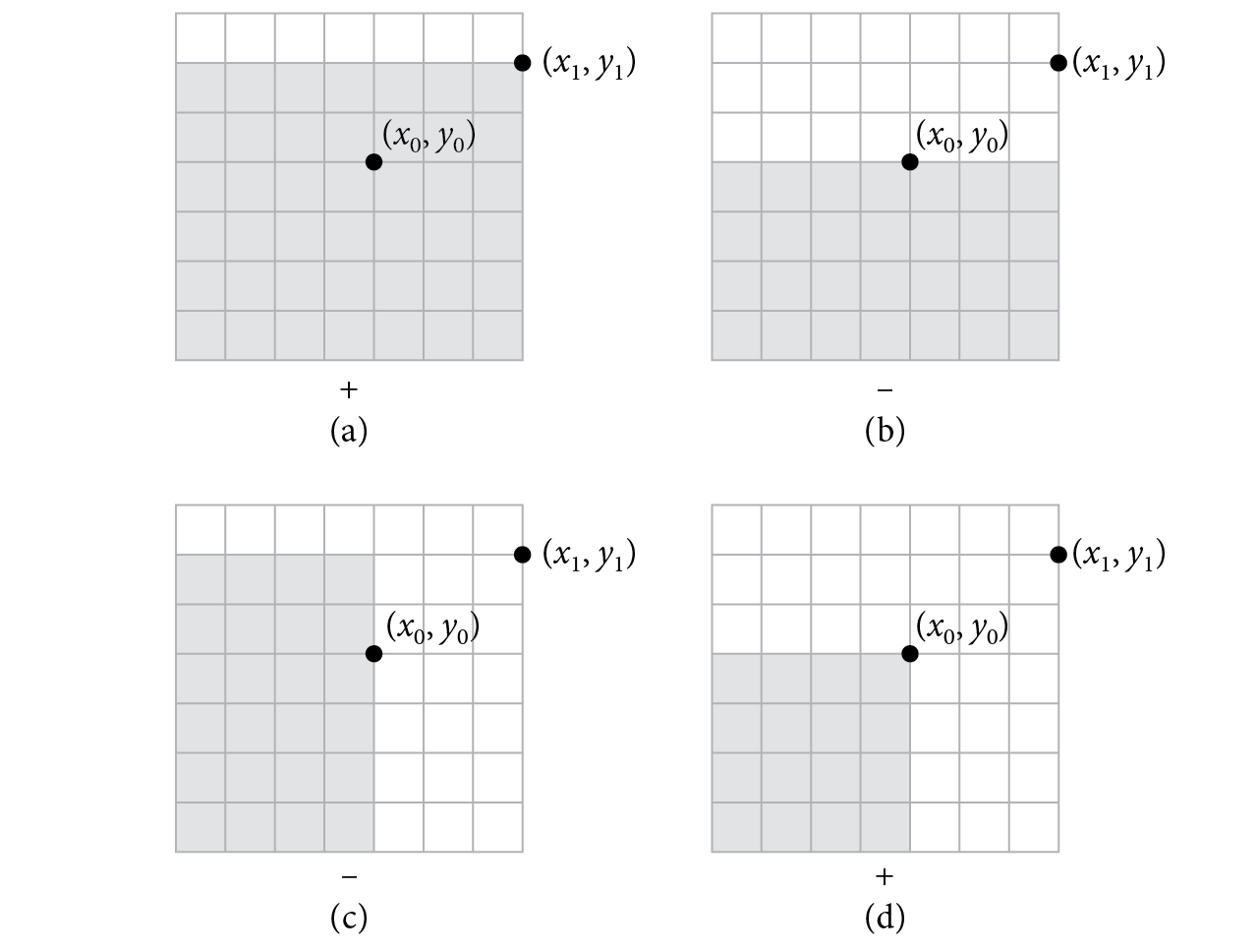
The remainder of the sums are computed incrementally by adding the corresponding value from the provided array to two of the previous sums and subtracting a third. It is possible to use the definition from Equation (A.17) to verify that this expression gives the desired value, but it can also be understood geometrically; see Figure A.12.

Figure A.12: Computing a Value in a Summed-Area Table Based on Previous Sums. (a) A starting value for the sum at a location left-parenthesis x comma y right-parenthesis (filled circle) is given by the sum at left-parenthesis x minus 1 comma y right-parenthesis (shaded region). To this value, we need to add the provided array’s value at left-parenthesis x comma y right-parenthesis . (b) What is left is the sum of values in the column beneath left-parenthesis x comma y right-parenthesis (lighter shaded region); that value can be found by taking the sum at left-parenthesis x comma y minus 1 right-parenthesis and subtracting the sum at left-parenthesis x minus 1 comma y minus 1 right-parenthesis (darker shaded region).

<<Compute sums for the remainder of the entries>>= 
for (int y = 1; y < sum.YSize(); ++y) for (int x = 1; x < sum.XSize(); ++x) sum(x, y) = (values(x, y) + sum(x - 1, y) + sum(x, y - 1) - sum(x - 1, y - 1));

Figure A.13: Interpretation of sum Array Values. If the sample array values is interpreted as defining a piecewise-constant function over left-bracket 0 comma 1 right-bracket squared , then the values stored in sum represent the sums at the upper-right corner of each piecewise-constant region. The sums along x equals 0 and y equals 0 , all of which are 0, are not stored.

We will find it useful to be able to treat the sum as a continuous function defined over left-bracket 0 comma 1 right-bracket squared . In doing so, our implementation effectively treats the originally provided array of values as the specification of a piecewise-constant function. Under this interpretation, the stored sum values effectively represent the function’s value at the upper corners of the box-shaped regions that the domain has been discretized into. (See Figure A.13.)

This Lookup() method returns the interpolated sum at the given continuous coordinate values.

<<SummedAreaTable Private Methods>>= 
Float Lookup(Float x, Float y) const { <<Rescale left-parenthesis x comma y right-parenthesis to table resolution and compute integer coordinates>> 
x *= sum.XSize(); y *= sum.YSize(); int x0 = (int)x, y0 = (int)y;
<<Bilinearly interpolate between surrounding table values>> 
Float v00 = LookupInt(x0, y0), v10 = LookupInt(x0 + 1, y0); Float v01 = LookupInt(x0, y0 + 1), v11 = LookupInt(x0 + 1, y0 + 1); Float dx = x - int(x), dy = y - int(y); return (1 - dx) * (1 - dy) * v00 + (1 - dx) * dy * v01 + dx * (1 - dy) * v10 + dx * dy * v11;
}

It is more convenient to work with coordinates that are with respect to the array’s dimensions and so this method starts by scaling the provided coordinates accordingly. Note that an offset of 0.5 is not included in this remapping, as is done when indexing pixel values (recall the discussion of this topic in Section 8.1.4); this is due to the fact that sum defines function values at the upper corners of the discretized regions rather than at their center.

<<Rescale left-parenthesis x comma y right-parenthesis to table resolution and compute integer coordinates>>= 
x *= sum.XSize(); y *= sum.YSize(); int x0 = (int)x, y0 = (int)y;

Bilinear interpolation of the four values surrounding the lookup point proceeds as usual, using LookupInt() to look up values of the sum at provided integer coordinates.

<<Bilinearly interpolate between surrounding table values>>= 
Float v00 = LookupInt(x0, y0), v10 = LookupInt(x0 + 1, y0); Float v01 = LookupInt(x0, y0 + 1), v11 = LookupInt(x0 + 1, y0 + 1); Float dx = x - int(x), dy = y - int(y); return (1 - dx) * (1 - dy) * v00 + (1 - dx) * dy * v01 + dx * (1 - dy) * v10 + dx * dy * v11;

LookupInt() returns the value of the sum for provided integer coordinates. In particular, it is responsible for handling the details related to the sum array storing the sum at the upper corners of the domain strata.

<<SummedAreaTable Private Methods>>+= 
Float LookupInt(int x, int y) const { <<Return zero at lower boundaries>> 
if (x == 0 || y == 0) return 0;
<<Reindex left-parenthesis x comma y right-parenthesis and return actual stored value>> 
x = std::min(x - 1, sum.XSize() - 1); y = std::min(y - 1, sum.YSize() - 1); return sum(x, y);
}

If either coordinate is zero-valued, the lookup point is along one of the lower edges of the domain (or is at the origin). In this case, a sum value of 0 is returned.

<<Return zero at lower boundaries>>= 
if (x == 0 || y == 0) return 0;

Otherwise, one is subtracted from each coordinate so that indexing into the sum array accounts for the zero sums at the lower edges not being stored in sum.

<<Reindex left-parenthesis x comma y right-parenthesis and return actual stored value>>= 
x = std::min(x - 1, sum.XSize() - 1); y = std::min(y - 1, sum.YSize() - 1); return sum(x, y);

Summed-area tables compute sums and integrals over arbitrary rectangular regions in a similar way to how the interior sum values were originally initialized. Here it is also possible to verify this computation algebraically, but the geometric interpretation may be more intuitive; see Figure A.14.

Figure A.14: Computing the Sum of an Arbitrary Rectangular Region. Given two points left-parenthesis x 0 comma y 0 right-parenthesis and left-parenthesis x 1 comma y 1 right-parenthesis representing the corners of a rectangular region, the sum of values inside the rectangular region can be found in terms of sums of subregions. (a) The sum at left-parenthesis x 1 comma y 1 right-parenthesis gives the desired result and then much more. (b) Subtracting the left-parenthesis x 0 comma y 1 right-parenthesis sum eliminates some of the excess, leaving the region underneath the region to be removed. (c) Subtracting the left-parenthesis x 1 comma y 0 right-parenthesis sum takes care of the excess and then some; the shaded region has now been removed twice. (d) Adding the shaded region’s sum, which is the sum at left-parenthesis x 0 comma y 0 right-parenthesis , rectifies the excess subtraction and leaves us with the desired result.

The SummedAreaTable class provides this capability through its Integral() method, which returns the integral of the piecewise-constant function over a 2D bounding box. Here, the sum of function values over the region is converted to an integral by dividing by the size of the function strata over the domain. We have used double precision here to compute the final sum in order to improve its accuracy: especially if there are thousands of values in each dimension, the sums may have large magnitudes and thus taking their differences can lead to catastrophic cancellation.

<<SummedAreaTable Public Methods>>+= 
Float Integral(Bounds2f extent) const { double s = (((double)Lookup(extent.pMax.x, extent.pMax.y) - (double)Lookup(extent.pMin.x, extent.pMax.y)) + ((double)Lookup(extent.pMin.x, extent.pMin.y) - (double)Lookup(extent.pMax.x, extent.pMin.y))); return std::max<Float>(s / (sum.XSize() * sum.YSize()), 0); }

Given SummedAreaTable’s capability of efficiently evaluating integrals over rectangular regions of a piecewise-constant function’s domain, the WindowedPiecewiseConstant2D class is able to provide sampling and PDF evaluation functions that operate over arbitrary caller-specified regions.

<<WindowedPiecewiseConstant2D Definition>>= 
class WindowedPiecewiseConstant2D { public: <<WindowedPiecewiseConstant2D Public Methods>> 
WindowedPiecewiseConstant2D(Array2D<Float> f, Allocator alloc = {}) : sat(f, alloc), func(f, alloc) {} pstd::optional<Point2f> Sample(Point2f u, Bounds2f b, Float *pdf) const { <<Handle zero-valued function for windowed sampling>> 
if (sat.Integral(b) == 0) return {};
<<Define lambda function Px for marginal cumulative distribution>> 
Float bInt = sat.Integral(b); auto Px = [&, this](Float x) -> Float { Bounds2f bx = b; bx.pMax.x = x; return sat.Integral(bx) / bInt; };
<<Sample marginal windowed function in x >> 
Point2f p; p.x = SampleBisection(Px, u[0], b.pMin.x, b.pMax.x, func.XSize());
<<Sample conditional windowed function in y >> 
<<Compute 2D bounds bCond for conditional sampling>> 
int nx = func.XSize(); Bounds2f bCond(Point2f(pstd::floor(p.x * nx) / nx, b.pMin.y), Point2f(pstd::ceil(p.x * nx) / nx, b.pMax.y)); if (bCond.pMin.x == bCond.pMax.x) bCond.pMax.x += 1.f / nx; if (sat.Integral(bCond) == 0) return {};
<<Define lambda function for conditional distribution and sample y >> 
Float condIntegral = sat.Integral(bCond); auto Py = [&, this](Float y) -> Float { Bounds2f by = bCond; by.pMax.y = y; return sat.Integral(by) / condIntegral; }; p.y = SampleBisection(Py, u[1], b.pMin.y, b.pMax.y, func.YSize());
<<Compute PDF and return point sampled from windowed function>> 
*pdf = Eval(p) / bInt; return p;
} Float PDF(Point2f p, const Bounds2f &b) const { Float funcInt = sat.Integral(b); if (funcInt == 0) return 0; return Eval(p) / funcInt; }
private: <<WindowedPiecewiseConstant2D Private Methods>> 
template <typename CDF> static Float SampleBisection(CDF P, Float u, Float min, Float max, int n) { <<Apply bisection to bracket u>> 
while (pstd::ceil(n * max) - pstd::floor(n * min) > 1) { Float mid = (min + max) / 2; if (P(mid) > u) max = mid; else min = mid; }
<<Find sample by interpolating between min and max>> 
Float t = (u - P(min)) / (P(max) - P(min)); return Clamp(Lerp(t, min, max), min, max);
} Float Eval(Point2f p) const { Point2i pi(std::min<int>(p[0] * func.XSize(), func.XSize() - 1), std::min<int>(p[1] * func.YSize(), func.YSize() - 1)); return func[pi]; }
<<WindowedPiecewiseConstant2D Private Members>> 
SummedAreaTable sat; Array2D<Float> func;
};

The constructor both copies the provided function values and initializes a summed-area table with them.

<<WindowedPiecewiseConstant2D Public Methods>>= 
WindowedPiecewiseConstant2D(Array2D<Float> f, Allocator alloc = {}) : sat(f, alloc), func(f, alloc) {}

<<WindowedPiecewiseConstant2D Private Members>>= 
SummedAreaTable sat; Array2D<Float> func;

With the SummedAreaTable in hand, it is now possible to bring the pieces together to implement the Sample() method. Because it is possible that there is no valid sample inside the specified bounds (e.g., if the function’s value is zero), an optional return value is used in order to be able to indicate such cases.

<<WindowedPiecewiseConstant2D Public Methods>>+=  
pstd::optional<Point2f> Sample(Point2f u, Bounds2f b, Float *pdf) const { <<Handle zero-valued function for windowed sampling>> 
if (sat.Integral(b) == 0) return {};
<<Define lambda function Px for marginal cumulative distribution>> 
Float bInt = sat.Integral(b); auto Px = [&, this](Float x) -> Float { Bounds2f bx = b; bx.pMax.x = x; return sat.Integral(bx) / bInt; };
<<Sample marginal windowed function in x >> 
Point2f p; p.x = SampleBisection(Px, u[0], b.pMin.x, b.pMax.x, func.XSize());
<<Sample conditional windowed function in y >> 
<<Compute 2D bounds bCond for conditional sampling>> 
int nx = func.XSize(); Bounds2f bCond(Point2f(pstd::floor(p.x * nx) / nx, b.pMin.y), Point2f(pstd::ceil(p.x * nx) / nx, b.pMax.y)); if (bCond.pMin.x == bCond.pMax.x) bCond.pMax.x += 1.f / nx; if (sat.Integral(bCond) == 0) return {};
<<Define lambda function for conditional distribution and sample y >> 
Float condIntegral = sat.Integral(bCond); auto Py = [&, this](Float y) -> Float { Bounds2f by = bCond; by.pMax.y = y; return sat.Integral(by) / condIntegral; }; p.y = SampleBisection(Py, u[1], b.pMin.y, b.pMax.y, func.YSize());
<<Compute PDF and return point sampled from windowed function>> 
*pdf = Eval(p) / bInt; return p;
}

The first step is to check whether the function’s integral is zero over the specified bounds. This may happen due to a degenerate Bounds2f or due to a plain old zero-valued function over the corresponding part of its domain. In this case, it is not possible to return a valid sample.

<<Handle zero-valued function for windowed sampling>>= 
if (sat.Integral(b) == 0) return {};

As discussed in Section 2.4.2, multidimensional distributions can be sampled by first integrating out all of the dimensions but one, sampling the resulting function, and then using that sample value in sampling the corresponding conditional distribution. WindowedPiecewiseConstant2D applies that very same idea, taking advantage of the fact that the summed-area table can efficiently evaluate the necessary integrals as needed.

For a 2D continuous function f left-parenthesis x comma y right-parenthesis defined over a rectangular domain from left-parenthesis x 0 comma y 0 right-parenthesis to left-parenthesis x 1 comma y 1 right-parenthesis , the marginal distribution in x is defined by

p left-parenthesis x right-parenthesis equals StartFraction integral Subscript y 0 Superscript y 1 Baseline f left-parenthesis x comma y Superscript prime Baseline right-parenthesis normal d y Superscript prime Baseline Over integral Subscript x 0 Superscript x 1 Baseline integral Subscript y 0 Superscript y 1 Baseline f left-parenthesis x prime comma y Superscript prime Baseline right-parenthesis normal d x prime normal d y Superscript prime Baseline EndFraction comma

and the marginal’s cumulative distribution is

upper P left-parenthesis x right-parenthesis equals StartFraction integral Subscript x 0 Superscript x Baseline integral Subscript y 0 Superscript y 1 Baseline f left-parenthesis x prime comma y Superscript prime Baseline right-parenthesis normal d x prime normal d y Superscript prime Baseline Over integral Subscript x 0 Superscript x 1 Baseline integral Subscript y 0 Superscript y 1 Baseline f left-parenthesis x prime comma y Superscript prime Baseline right-parenthesis normal d x prime normal d y Superscript prime Baseline EndFraction period

The integrals in both the numerator and denominator of upper P left-parenthesis x right-parenthesis can be evaluated using a summed-area table. The following lambda function evaluates upper P left-parenthesis x right-parenthesis , using a cached normalization factor for the denominator in bInt to improve performance, as it will be necessary to repeatedly evaluate Px in order to sample from the distribution.

<<Define lambda function Px for marginal cumulative distribution>>= 
Float bInt = sat.Integral(b); auto Px = [&, this](Float x) -> Float { Bounds2f bx = b; bx.pMax.x = x; return sat.Integral(bx) / bInt; };

Sampling is performed using a separate utility method, SampleBisection(), that will also be useful for sampling the conditional density in y .

<<Sample marginal windowed function in x >>= 
Point2f p; p.x = SampleBisection(Px, u[0], b.pMin.x, b.pMax.x, func.XSize());

SampleBisection() draws a sample from the density described by the provided CDF P by applying the bisection method to solve u equals upper P left-parenthesis x right-parenthesis for x over a specified range left-bracket monospace m monospace i monospace n monospace comma monospace m monospace a monospace x monospace right-bracket . (It expects upper P left-parenthesis x right-parenthesis to have the value 0 at min and 1 at max.) This function has the built-in assumption that the CDF is piecewise-linear over n equal-sized segments over left-bracket 0 comma 1 right-bracket . This fits SummedAreaTable perfectly, though it means that SampleBisection() would need modification to be used in other contexts.

<<WindowedPiecewiseConstant2D Private Methods>>= 
template <typename CDF> static Float SampleBisection(CDF P, Float u, Float min, Float max, int n) { <<Apply bisection to bracket u>> 
while (pstd::ceil(n * max) - pstd::floor(n * min) > 1) { Float mid = (min + max) / 2; if (P(mid) > u) max = mid; else min = mid; }
<<Find sample by interpolating between min and max>> 
Float t = (u - P(min)) / (P(max) - P(min)); return Clamp(Lerp(t, min, max), min, max);
}

The initial min and max values bracket the solution. Therefore, bisection can proceed by successively evaluating upper P at their midpoint and then updating one or the other of them to maintain the bracket. This process continues until both endpoints lie inside one of the function discretization strata of width 1 slash n .

<<Apply bisection to bracket u>>= 
while (pstd::ceil(n * max) - pstd::floor(n * min) > 1) { Float mid = (min + max) / 2; if (P(mid) > u) max = mid; else min = mid; }

Once both endpoints are in the same stratum, it is possible to take advantage of the fact that upper P is known to be piecewise-linear and to find the value of x in closed form.

<<Find sample by interpolating between min and max>>= 
Float t = (u - P(min)) / (P(max) - P(min)); return Clamp(Lerp(t, min, max), min, max);

Given the sample x , we now need to draw a sample from the conditional distribution

p left-parenthesis y vertical-bar x right-parenthesis equals StartFraction f left-parenthesis x comma y right-parenthesis Over integral Subscript y 0 Superscript y 1 Baseline f left-parenthesis x comma y Superscript prime Baseline right-parenthesis normal d y Superscript prime Baseline EndFraction comma

which has CDF

upper P left-parenthesis y vertical-bar x right-parenthesis equals StartFraction integral Subscript y 0 Superscript y Baseline f left-parenthesis x comma y Superscript prime Baseline right-parenthesis normal d y Superscript prime Baseline Over integral Subscript y 0 Superscript y 1 Baseline f left-parenthesis x comma y Superscript prime Baseline right-parenthesis normal d y Superscript prime Baseline EndFraction period

Although the SummedAreaTable class does not provide the capability to evaluate 1D integrals directly, because the function is piecewise-constant we can equivalently evaluate a 2D integral where the x range spans only the stratum of the sampled x value.

<<Sample conditional windowed function in y >>= 
<<Compute 2D bounds bCond for conditional sampling>> 
int nx = func.XSize(); Bounds2f bCond(Point2f(pstd::floor(p.x * nx) / nx, b.pMin.y), Point2f(pstd::ceil(p.x * nx) / nx, b.pMax.y)); if (bCond.pMin.x == bCond.pMax.x) bCond.pMax.x += 1.f / nx; if (sat.Integral(bCond) == 0) return {};
<<Define lambda function for conditional distribution and sample y >> 
Float condIntegral = sat.Integral(bCond); auto Py = [&, this](Float y) -> Float { Bounds2f by = bCond; by.pMax.y = y; return sat.Integral(by) / condIntegral; }; p.y = SampleBisection(Py, u[1], b.pMin.y, b.pMax.y, func.YSize());

bCond stores the bounding box that spans the range of potential y values and the stratum of the x sample. It is necessary to check for a zero function integral over these bounds: this should not be possible mathematically, but may be the case due to floating-point round-off error. In that rare case, conditional sampling is not possible and an invalid sample must be returned.

<<Compute 2D bounds bCond for conditional sampling>>= 
int nx = func.XSize(); Bounds2f bCond(Point2f(pstd::floor(p.x * nx) / nx, b.pMin.y), Point2f(pstd::ceil(p.x * nx) / nx, b.pMax.y)); if (bCond.pMin.x == bCond.pMax.x) bCond.pMax.x += 1.f / nx; if (sat.Integral(bCond) == 0) return {};

Similar to the marginal CDF upper P left-parenthesis x right-parenthesis , we can define a lambda function to evaluate the conditional CDF upper P left-parenthesis y vertical-bar x right-parenthesis . Again precomputing the normalization factor is worthwhile, as Py will be evaluated multiple times in the course of the sampling operation.

<<Define lambda function for conditional distribution and sample y >>= 
Float condIntegral = sat.Integral(bCond); auto Py = [&, this](Float y) -> Float { Bounds2f by = bCond; by.pMax.y = y; return sat.Integral(by) / condIntegral; }; p.y = SampleBisection(Py, u[1], b.pMin.y, b.pMax.y, func.YSize());

The PDF value is computed by evaluating the function at the sampled point p and normalizing with its integral over b, which is already available in bInt.

<<Compute PDF and return point sampled from windowed function>>= 
*pdf = Eval(p) / bInt; return p;

The Eval() method wraps up the details of looking up the function value corresponding to the provided 2D point.

<<WindowedPiecewiseConstant2D Private Methods>>+= 
Float Eval(Point2f p) const { Point2i pi(std::min<int>(p[0] * func.XSize(), func.XSize() - 1), std::min<int>(p[1] * func.YSize(), func.YSize() - 1)); return func[pi]; }

The PDF method implements the same computation that is used to compute the PDF in the Sample() method.

<<WindowedPiecewiseConstant2D Public Methods>>+= 
Float PDF(Point2f p, const Bounds2f &b) const { Float funcInt = sat.Integral(b); if (funcInt == 0) return 0; return Eval(p) / funcInt; }