8.1 Sampling Theory
A digital image is represented as a set of pixel values, typically aligned on a rectangular grid. When a digital image is displayed on a physical device, these values are used to determine the spectral power emitted by pixels on the display. When thinking about digital images, it is important to differentiate between image pixels, which represent the value of a function at a particular sample location, and display pixels, which are physical objects that emit light with some spatial and directional distribution. (For example, in an LCD display, the color and brightness may change substantially when the display is viewed at oblique angles.) Displays use the image pixel values to construct a new image function over the display surface. This function is defined at all points on the display, not just the infinitesimal points of the digital image’s pixels. This process of taking a collection of sample values and converting them back to a continuous function is called reconstruction.
In order to compute the discrete pixel values in the digital image, it is necessary to sample the original continuously defined image function. In pbrt, like most other ray-tracing renderers, the only way to get information about the image function is to sample it by tracing rays. For example, there is no general method that can compute bounds on the variation of the image function between two points on the film plane. While an image could be generated by just sampling the function precisely at the pixel positions, a better result can be obtained by taking more samples at different positions and incorporating this additional information about the image function into the final pixel values. Indeed, for the best quality result, the pixel values should be computed such that the reconstructed image on the display device is as close as possible to the original image of the scene on the virtual camera’s film plane. Note that this is a subtly different goal from expecting the display’s pixels to take on the image function’s actual value at their positions. Handling this difference is the main goal of the algorithms implemented in this chapter.
Because the sampling and reconstruction process involves approximation, it introduces error known as aliasing, which can manifest itself in many ways, including jagged edges or flickering in animations. These errors occur because the sampling process is not able to capture all the information from the continuously defined image function.
As an example of these ideas, consider a 1D function (which we will interchangeably refer to as a signal), given by , where we can evaluate at any desired location in the function’s domain. Each such is called a sample position, and the value of is the sample value. Figure 8.1 shows a set of samples of a smooth 1D function, along with a reconstructed signal that approximates the original function . In this example, is a piecewise linear function that approximates by linearly interpolating neighboring sample values (readers already familiar with sampling theory will recognize this as reconstruction with a hat function). Because the only information available about comes from the sample values at the positions , is unlikely to match perfectly since there is no information about ’s behavior between the samples.

Fourier analysis can be used to evaluate the quality of the match between the reconstructed function and the original. This section will introduce the main ideas of Fourier analysis with enough detail to work through some parts of the sampling and reconstruction processes but will omit proofs of many properties and skip details that are not directly relevant to the sampling algorithms used in pbrt. The “Further Reading” section of this chapter has pointers to more detailed information about these topics.
8.1.1 The Frequency Domain and the Fourier Transform
One of the foundations of Fourier analysis is the Fourier transform, which represents a function in the frequency domain. (We will say that functions are normally expressed in the spatial domain.) Consider the two functions graphed in Figure 8.2. The function in Figure 8.2(a) varies relatively slowly as a function of , while the function in Figure 8.2(b) varies much more rapidly. The more slowly varying function is said to have lower-frequency content.

Figure 8.3 shows the frequency space representations of these two functions; the lower-frequency function’s representation goes to 0 more quickly than does the higher-frequency function.

Most functions can be decomposed into a weighted sum of shifted sinusoids. This remarkable fact was first described by Joseph Fourier, and the Fourier transform converts a function into this representation. This frequency space representation of a function gives insight into some of its characteristics—the distribution of frequencies in the sine functions corresponds to the distribution of frequencies in the original function. Using this form, it is possible to use Fourier analysis to gain insight into the error that is introduced by the sampling and reconstruction process and how to reduce the perceptual impact of this error.
The Fourier transform of a 1D function is
(Recall that , where .) For simplicity, here we will consider only even functions where , in which case the Fourier transform of has no imaginary terms. The new function is a function of frequency, . We will denote the Fourier transform operator by , such that . is clearly a linear operator—that is, for any scalar , and . The Fourier transform has a straightforward generalization to multidimensional functions where is a corresponding multidimensional value, though we will generally stick to the 1D case for notational simplicity.
Equation (8.1) is called the Fourier analysis equation, or sometimes just the Fourier transform. We can also transform from the frequency domain back to the spatial domain using the Fourier synthesis equation, or the inverse Fourier transform:
Table 8.1 shows a number of important functions and their frequency space representations. A number of these functions are based on the Dirac delta distribution, which is defined such that , and for all , . An important consequence of these properties is that
The delta distribution cannot be expressed as a standard mathematical function, but instead is generally thought of as the limit of a unit area box function centered at the origin with width approaching 0.
| Spatial Domain | Frequency Space Representation |
|---|---|
| Box: if , otherwise | Sinc: |
| Gaussian: | Gaussian: |
| Constant: | Delta: |
| Sinusoid: | Translated delta: |
| Shah: | Shah: |
8.1.2 Ideal Sampling and Reconstruction
Using frequency space analysis, we can now formally investigate the properties of sampling. Recall that the sampling process requires us to choose a set of equally spaced sample positions and compute the function’s value at those positions. Formally, this corresponds to multiplying the function by a “shah,” or “impulse train,” function, an infinite sum of equally spaced delta functions. The shah is defined as
where defines the period, or sampling rate. This formal definition of sampling is illustrated in Figure 8.4. The multiplication yields an infinite sequence of values of the function at equally spaced points:

These sample values can be used to define a reconstructed function by choosing a reconstruction filter function and computing the convolution
where the convolution operation is defined as
For reconstruction, convolution gives a weighted sum of scaled instances of the reconstruction filter centered at the sample points:
For example, in Figure 8.1, the triangle reconstruction filter, , was used. Figure 8.5 shows the scaled triangle functions used for that example.

We have gone through a process that may seem gratuitously complex in order to end up at an intuitive result: the reconstructed function can be obtained by interpolating among the samples in some manner. By setting up this background carefully, however, we can now apply Fourier analysis to the process more easily.
We can gain a deeper understanding of the sampling process by analyzing the sampled function in the frequency domain. In particular, we will be able to determine the conditions under which the original function can be exactly recovered from its values at the sample locations—a very powerful result. For the discussion here, we will assume for now that the function is band limited—there exists some frequency such that contains no frequencies greater than . By definition, band-limited functions have frequency space representations with compact support, such that for all . Both of the spectra in Figure 8.3 are band limited.
An important idea used in Fourier analysis is the fact that the Fourier transform of the product of two functions can be shown to be the convolution of their individual Fourier transforms and :
It is similarly the case that convolution in the spatial domain is equivalent to multiplication in the frequency domain:
These properties are derived in the standard references on Fourier analysis. Using these ideas, the original sampling step in the spatial domain, where the product of the shah function and the original function is found, can be equivalently described by the convolution of with another shah function in frequency space.
We also know the spectrum of the shah function from Table 8.1; the Fourier transform of a shah function with period is another shah function with period . This reciprocal relationship between periods is important to keep in mind: it means that if the samples are farther apart in the spatial domain, they are closer together in the frequency domain.
Thus, the frequency domain representation of the sampled signal is given by the convolution of and this new shah function. Convolving a function with a delta function just yields a copy of the function, so convolving with a shah function yields an infinite sequence of copies of the original function, with spacing equal to the period of the shah (Figure 8.6). This is the frequency space representation of the series of samples.

Now that we have this infinite set of copies of the function’s spectrum, how do we reconstruct the original function? Looking at Figure 8.6, the answer is obvious: just discard all of the spectrum copies except the one centered at the origin, giving the original .

In order to throw away all but the center copy of the spectrum, we multiply by a box function of the appropriate width (Figure 8.7). The box function of width is defined as
This multiplication step corresponds to convolution with the reconstruction filter in the spatial domain. This is the ideal sampling and reconstruction process. To summarize:
This is a remarkable result: we have been able to determine the exact frequency space representation of , purely by sampling it at a set of regularly spaced points. Other than knowing that the function was band limited, no additional information about the composition of the function was used.
Applying the equivalent process in the spatial domain will likewise recover exactly. Because the inverse Fourier transform of the box function is the sinc function, ideal reconstruction in the spatial domain is
where , and thus
Unfortunately, because the sinc function has infinite extent, it is necessary to use all the sample values to compute any particular value of in the spatial domain. Filters with finite spatial extent are preferable for practical implementations even though they do not reconstruct the original function perfectly.
A commonly used alternative in graphics is to use the box function for reconstruction, effectively averaging all the sample values within some region around . This is a poor choice, as can be seen by considering the box filter’s behavior in the frequency domain: This technique attempts to isolate the central copy of the function’s spectrum by multiplying by a sinc, which not only does a bad job of selecting the central copy of the function’s spectrum but includes high-frequency contributions from the infinite series of other copies of it as well.
8.1.3 Aliasing
Beyond the issue of the sinc function’s infinite extent, one of the most serious practical problems with the ideal sampling and reconstruction approach is the assumption that the signal is band limited. For signals that are not band limited, or signals that are not sampled at a sufficiently high sampling rate for their frequency content, the process described earlier will reconstruct a function that is different from the original signal. Both the underlying problem and mitigation strategies for it can be understood using Fourier analysis.
The key to successful reconstruction is the ability to exactly recover the original spectrum by multiplying the sampled spectrum with a box function of the appropriate width. Notice that in Figure 8.6, the copies of the signal’s spectrum are separated by empty space, so perfect reconstruction is possible. Consider what happens, however, if the original function was sampled with a lower sampling rate. Recall that the Fourier transform of a shah function with period is a new shah function with period . This means that if the spacing between samples increases in the spatial domain, the sample spacing decreases in the frequency domain, pushing the copies of the spectrum closer together. If the copies get too close together, they start to overlap.
Because the copies are added together, the resulting spectrum no longer looks like many copies of the original (Figure 8.8). When this new spectrum is multiplied by a box function, the result is a spectrum that is similar but not equal to the original : high-frequency details in the original signal leak into lower-frequency regions of the spectrum of the reconstructed signal. These new low-frequency artifacts are called aliases (because high frequencies are “masquerading” as low frequencies), and the resulting signal is said to be aliased. It is sometimes useful to distinguish between artifacts due to sampling and those due to reconstruction; when we wish to be precise we will call sampling artifacts prealiasing and reconstruction artifacts postaliasing. Any attempt to fix these errors is broadly classified as antialiasing.

Figure 8.9 shows the effects of aliasing from undersampling and then reconstructing the 1D function .

A possible solution to the problem of overlapping spectra is to simply increase the sampling rate until the copies of the spectrum are sufficiently far apart not to overlap, thereby eliminating aliasing completely. The sampling theorem tells us exactly what rate is required. This theorem says that as long as the frequency of uniformly spaced sample points is greater than twice the maximum frequency present in the signal , it is possible to reconstruct the original signal perfectly from the samples. This minimum sampling frequency is called the Nyquist frequency.
However, increasing the sampling rate is expensive in a ray tracer: the time to render an image is directly proportional to the number of samples taken. Furthermore, for signals that are not band limited (), it is impossible to sample at a high enough rate to perform perfect reconstruction. Non-band-limited signals have spectra with infinite support, so no matter how far apart the copies of their spectra are (i.e., how high a sampling rate we use), there will always be overlap.
Unfortunately, few of the interesting functions in computer graphics are band limited. In particular, any function containing a discontinuity cannot be band limited, and therefore we cannot perfectly sample and reconstruct it. This makes sense because the function’s discontinuity will always fall between two samples and the samples provide no information about the location of the discontinuity. Thus, it is necessary to apply different methods besides just increasing the sampling rate in order to counteract the error that aliasing can introduce to the renderer’s results.
8.1.4 Understanding Pixels
With this understanding of sampling and reconstruction in mind, it is worthwhile to establish some terminology and conventions related to pixels.
The word “pixel” is used to refer to two different things: physical elements that either emit or measure light (as used in displays and digital cameras) and regular samples of an image function (as used for image textures, for example). Although the pixels in an image may be measured by the pixels in a camera’s sensor, and although the pixels in an image may be used to set the emission from pixels in a display, it is important to be attentive to the differences between them.
The pixels that constitute an image are defined to be point samples of an image function at discrete points on the image plane; there is no “area” associated with an image pixel. As Alvy Ray Smith (1995) has emphatically pointed out, thinking of the pixels in an image as small squares with finite area is an incorrect mental model that leads to a series of errors. We may filter the continuously defined image function over an area to compute an image pixel value, though we will maintain the distinction in that case that a pixel represents a point sample of a filtered function.
A related issue is that the pixels in an image are naturally defined at discrete integer coordinates on a pixel grid, but it will often be useful to consider an image as a continuous function of positions. The natural way to map between these two domains is to round continuous coordinates to the nearest discrete coordinate; doing so is appealing since it maps continuous coordinates that happen to have the same value as discrete coordi- nates to that discrete coordinate. However, the result is that given a set of discrete coor- dinates spanning a range , the set of continuous coordinates that covers that range is . Thus, any code that generates continuous sample positions for a given discrete pixel range is littered with offsets. It is easy to forget some of these, leading to subtle errors.
A better convention is to truncate continuous coordinates to discrete coordinates by
and convert from discrete to continuous by
In this case, the range of continuous coordinates for the discrete range is naturally , and the resulting code is much simpler (Heckbert 1990a). This convention, which we have adopted in pbrt, is shown graphically in Figure 8.10.

8.1.5 Sampling and Aliasing in Rendering
The application of the principles of sampling theory to the 2D case of sampling and reconstructing images of rendered scenes is straightforward: we have an image, which we can think of as a function of 2D image locations to radiance values :
It is useful to generalize the definition of the scene function to a higher-dimensional function that also depends on the time and lens position at which it is sampled. Because the rays from the camera are based on these five quantities, varying any of them gives a different ray and thus a potentially different value of . For a particular image position, the radiance at that point will generally vary across both time (if there are moving objects in the scene) and position on the lens (if the camera has a finite-aperture lens).
Even more generally, because the integrators defined in Chapters 13 through 15 use Monte Carlo integration to estimate the radiance along a given ray, they may return a different radiance value when repeatedly given the same ray. If we further extend the scene radiance function to include sample values used by the integrator (e.g., values used to choose points on area light sources for illumination computations), we have an even higher-dimensional image function
Sampling all of these dimensions well is an important part of generating high-quality imagery efficiently. For example, if we ensure that nearby positions on the image tend to have dissimilar positions on the lens, the resulting rendered images will have less error because each sample is more likely to account for information about the scene that its neighboring samples do not. The Sampler class implementations later in this chapter will address the issue of sampling all of these dimensions effectively.
Sources of Aliasing

Geometry is one of the most common causes of aliasing in rendered images. When projected onto the image plane, an object’s boundary introduces a step function—the image function’s value instantaneously jumps from one value to another. Not only do step functions have infinite frequency content as mentioned earlier, but, even worse, the perfect reconstruction filter causes artifacts when applied to aliased samples: ringing artifacts appear in the reconstructed function, an effect known as the Gibbs phenomenon. Figure 8.11 shows an example of this effect for a 1D function. Choosing an effective reconstruction filter in the face of aliasing requires a mix of science, artistry, and personal taste, as we will see later in this chapter.
Very small objects in the scene can also cause geometric aliasing. If the geometry is small enough that it falls between samples on the image plane, it can unpredictably disappear and reappear over multiple frames of an animation.
Another source of aliasing can come from the texture and materials on an object. Shading aliasing can be caused by textures that have not been filtered correctly (addressing this problem is the topic of much of Chapter 10) or from small highlights on shiny surfaces. If the sampling rate is not high enough to sample these features adequately, aliasing will result. Furthermore, a sharp shadow cast by an object introduces another step function in the final image. While it is possible to identify the position of step functions from geometric edges on the image plane, detecting step functions from shadow boundaries is more difficult.
The inescapable conclusion about aliasing in rendered images is that we can never remove all of its sources, so we must develop techniques to mitigate its impact on the quality of the final image.
Adaptive Sampling
One approach that has been applied to combat aliasing is adaptive supersampling: if we can identify the regions of the signal with frequencies higher than the Nyquist limit, we can take additional samples in those regions without needing to incur the computational expense of increasing the sampling frequency everywhere. It can be difficult to get this approach to work well in practice, because finding all the places where supersampling is needed is difficult. Most techniques for doing so are based on examining adjacent sample values and finding places where there is a significant change in value between the two; the assumption is that the signal has high frequencies in that region.
In general, adjacent sample values cannot tell us with certainty what is really happening between them: even if the values are the same, the functions may have huge variation between them. Alternatively, adjacent samples may have substantially different values without any aliasing actually being present. For example, the texture-filtering algorithms in Chapter 10 work hard to eliminate aliasing due to image maps and procedural textures on surfaces in the scene; we would not want an adaptive sampling routine to needlessly take extra samples in an area where texture values are changing quickly but no excessively high frequencies are actually present.
Prefiltering
Another approach to eliminating aliasing that sampling theory offers is to filter (i.e., blur) the original function so that no high frequencies remain that cannot be captured accurately at the sampling rate being used. This approach is applied in the texture functions of Chapter 10. While this technique changes the character of the function being sampled by removing information from it, blurring is generally less objectionable than aliasing.
Recall that we would like to multiply the original function’s spectrum with a box filter with width chosen so that frequencies above the Nyquist limit are removed. In the spatial domain, this corresponds to convolving the original function with a sinc filter,
In practice, we can use a filter with finite extent that works well. The frequency space representation of this filter can help clarify how well it approximates the behavior of the ideal sinc filter.
Figure 8.12 shows the function convolved with a variant of the sinc with finite extent that will be introduced in Section 8.8. Note that the high-frequency details have been eliminated; this function can be sampled and reconstructed at the sampling rate used in Figure 8.9 without aliasing.

8.1.6 Spectral Analysis of Sampling Patterns
Given a fixed sampling rate, the remaining option to improve image quality is to consider how the distribution of sample positions affects the result. We can understand the behavior of deterministic sampling patterns like the shah function in frequency space by considering the convolution of its frequency space representation with a function’s frequency space representation. However, we will find it worthwhile to consider stochastic sampling methods where the sample positions are specified by one or more random variables. In that case, we will distinguish between the statistical properties of all the sets of samples that the algorithm may generate and a single set of points generated by it (which we will call a sample pattern); the former gives much more insight about an algorithm’s behavior.
A concept known as the power spectral density (PSD) is helpful for this task. For a function that is represented by in the Fourier basis, the PSD is defined as:
where is the complex conjugate of . (Under the assumption of an even function , .) Because the PSD discards information about the phase of the signal, the original Fourier coefficients cannot be recovered from it.
A useful property of the PSD is that the PSD of the product of two functions and in the spatial domain is given by the convolution of their PSDs in the Fourier domain:
This property follows directly from Equation (8.3). Therefore, if we have a point-sampling technique represented by a function that is defined as a sum of Dirac delta distributions (as the shah function was), then the frequency content from sampling a function is given by the convolution of and .
In some cases, the PSD of a sampling pattern can be derived analytically: doing so is easy for uniform random sampling, for example. For stochastic sampling patterns without an analytic PSD, the PSD can be computed numerically by averaging over random instances of the sample points. Because each sample point is represented as a Dirac delta distribution, their Fourier transform, Equation (8.1), ends up as a sum over the sample points.
The ideal sampling pattern’s PSD would have a single delta distribution spike at the origin and be zero everywhere else: in that case, sampling would exactly replicate . Unfortunately, such a sampling pattern would require an infinite sampling density. (This can be understood by considering the inverse Fourier transform of , which is a constant function.)
The PSD makes it possible to analyze the effects of stochastic sampling. One way to do so is through jittering, which adds uniform random offsets to regularly spaced sample points. With a uniform random number between 0 and 1, a random set of samples based on the impulse train is
It is possible to derive the expectation of the analytic PSD of this sampling strategy,
This function is graphed in Figure 8.13. Note that there is a spike at the origin, that its value is otherwise close to 0 in the low frequencies, and that it settles in to an increasingly narrow range around 1 at the higher frequencies.

We can use the PSD to compare the effect of undersampling a function in two different ways: using regularly spaced samples and using jittered samples. Figure 8.14(a) shows the frequency space representation of a function with energy in frequencies , which is the maximum frequency content that can be perfectly reconstructed with regular sampling with . Figure 8.14(b) then shows the result of convolving the function’s PSD with regular samples and Figure 8.14(c) shows the result with jittered samples.

In general, aliasing is reduced most effectively if there is minimal energy in the PSD of the sampling function at low frequencies. This characteristic prevents higher frequencies in the function being sampled from appearing as aliases at lower frequencies. (It is implicit in this assumption that the function ’s energy is concentrated in the lower frequencies. This is the case for most natural images, though if this is not the case, then the behavior of the sampling function’s PSD at the lower frequencies does not matter as much.)
While the shah function is effective by this measure, the uniformity of its sampling rate can lead to structured error, as was shown in Figure 8.14. With jittered sampling, the copies of the sampled signal end up being randomly shifted, so that when reconstruction is performed the result is random error rather than coherent aliasing. Because jittered sampling has roughly the same amount of energy in all the higher frequencies of its PSD, it spreads high-frequency energy in the function being sampled over many frequencies, converting aliasing into high-frequency noise, which is more visually pleasing to human observers than lower-frequency aliasing.
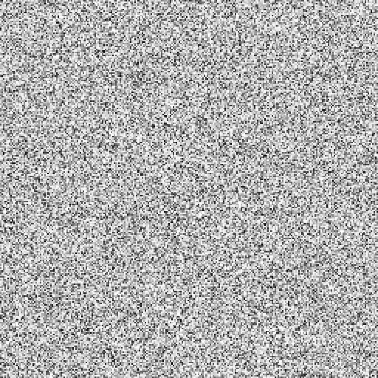
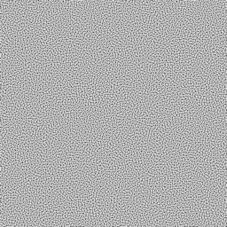
PSDs are sometimes described in terms of their color. For example, a white noise distribution has equal power at all frequencies, just as white light has (more or less) equal power at all visible frequencies. Blue noise corresponds to a distribution with its power concentrated at the higher frequencies and less power at low frequencies, again corresponding to the relationship between power and frequency exhibited by blue light.
We will occasionally find precomputed 2D tables of values that have blue noise characteristics to be useful; pbrt includes a number of such tables that are made available through the following function. Tables are reused once the provided tableIndex value goes past their number.
Figure 8.15 shows one such table along with a white noise image. With a blue noise distribution, the values at nearby pixels differ, corresponding to higher-frequency variation. Because the white noise image does not have this characteristic, there are visible clumps of pixels with similar values.