14.1 The Equation of Transfer

The equation of transfer is the fundamental equation that governs the behavior of light in a medium that absorbs, emits, and scatters radiation. It accounts for all the volume scattering processes described in Chapter 11—absorption, emission, in scattering, and out scattering—to give an equation that describes the equilibrium distribution of radiance. The light transport equation is in fact a special case of it, simplified by the lack of participating media and specialized for scattering from surfaces. (We will equivalently refer to the equation of transfer as the volumetric light transport equation.)

In its most basic form, the equation of transfer is an integro-differential equation that describes how the radiance along a beam changes at a point in space. It can be derived by subtracting the effects of the scattering processes that reduce energy along a beam (absorption and out scattering) from the processes that increase energy along it (emission and in scattering).

To start, recall the source function upper L Subscript normal s from Section 11.1.4: it gives the change in radiance at a point normal p Subscript in a direction omega Subscript due to emission and in-scattered light from other points in the medium:

upper L Subscript normal s Superscript Baseline left-parenthesis normal p Subscript Baseline comma omega Subscript Baseline right-parenthesis equals StartFraction sigma Subscript normal a Baseline left-parenthesis normal p Subscript Baseline comma omega Subscript Baseline right-parenthesis Over sigma Subscript normal t Baseline left-parenthesis normal p Subscript Baseline comma omega Subscript Baseline right-parenthesis EndFraction upper L Subscript normal e Baseline left-parenthesis normal p Subscript Baseline comma omega Subscript Baseline right-parenthesis plus StartFraction sigma Subscript normal s Baseline left-parenthesis normal p Subscript Baseline comma omega Subscript Baseline right-parenthesis Over sigma Subscript normal t Baseline left-parenthesis normal p Subscript Baseline comma omega Subscript Baseline right-parenthesis EndFraction integral Underscript script upper S squared Endscripts p left-parenthesis normal p Subscript Baseline comma omega Subscript normal i Baseline comma omega right-parenthesis upper L Subscript normal i Baseline left-parenthesis normal p Subscript Baseline comma omega Subscript normal i Baseline right-parenthesis normal d omega Subscript normal i Baseline period

The source function accounts for all the processes that add radiance to a ray.

The attenuation coefficient, sigma Subscript normal t Baseline left-parenthesis normal p Subscript Baseline comma omega Subscript Baseline right-parenthesis , accounts for all processes that reduce radiance at a point: absorption and out scattering. The differential equation that describes its effect, Equation (11.4), is

normal d upper L Subscript normal o Baseline left-parenthesis normal p Subscript Baseline comma omega Subscript Baseline right-parenthesis equals minus sigma Subscript normal t Baseline left-parenthesis normal p Subscript Baseline comma omega Subscript Baseline right-parenthesis upper L Subscript normal i Baseline left-parenthesis normal p Subscript Baseline comma minus omega Subscript Baseline right-parenthesis normal d t period

The overall differential change in radiance at a point normal p prime equals normal p Subscript Baseline plus t omega Subscript along a ray is found by adding these two effects together to get the integro-differential form of the equation of transfer:

StartFraction partial-differential Over partial-differential t EndFraction upper L Subscript normal o Baseline left-parenthesis normal p prime comma omega Subscript Baseline right-parenthesis equals minus sigma Subscript normal t Baseline left-parenthesis normal p prime comma omega Subscript Baseline right-parenthesis upper L Subscript normal i Baseline left-parenthesis normal p prime comma minus omega Subscript Baseline right-parenthesis plus sigma Subscript normal t Baseline left-parenthesis normal p prime comma omega Subscript Baseline right-parenthesis upper L Subscript normal s Superscript Baseline left-parenthesis normal p prime comma omega Subscript Baseline right-parenthesis period

(The sigma Subscript normal t modulation of the source function accounts for the medium’s density at the point.)

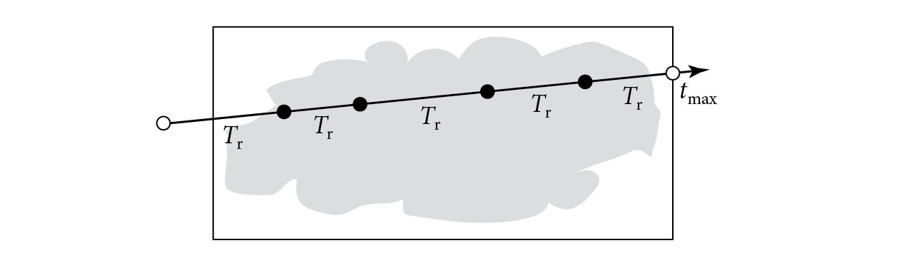
With suitable boundary conditions, this equation can be transformed to a pure integral equation that describes the effect of participating media from the infinite number of points along a ray. For example, if we assume that there are no surfaces in the scene so that the rays are never blocked and have an infinite length, the integral equation of transfer is

upper L Subscript normal i Baseline left-parenthesis normal p Subscript Baseline comma omega Subscript Baseline right-parenthesis equals integral Subscript 0 Superscript normal infinity Baseline upper T Subscript normal r Baseline left-parenthesis normal p prime right-arrow normal p Subscript Baseline right-parenthesis sigma Subscript normal t Baseline left-parenthesis normal p prime comma omega Subscript Baseline right-parenthesis upper L Subscript normal s Superscript Baseline left-parenthesis normal p prime comma minus omega Subscript Baseline right-parenthesis normal d t period

(See Figure 14.1.) The meaning of this equation is reasonably intuitive: it just says that the radiance arriving at a point from a given direction is determined by accumulating the radiance added at all points along the ray. The amount of added radiance at each point along the ray that reaches the ray’s origin is reduced by the beam transmittance to the point.

Figure 14.1: The equation of transfer gives the incident radiance at point upper L Subscript normal i Baseline left-parenthesis normal p Subscript Baseline comma omega Subscript Baseline right-parenthesis accounting for the effect of participating media. At each point normal p prime along the ray, the source function upper L Subscript normal s Superscript Baseline left-parenthesis normal p prime comma minus omega Subscript Baseline right-parenthesis gives the differential radiance added at the point due to scattering and emission. This radiance is then attenuated by the beam transmittance upper T Subscript r Baseline left-parenthesis normal p prime right-arrow normal p Subscript Baseline right-parenthesis from the point normal p prime to the ray’s origin.

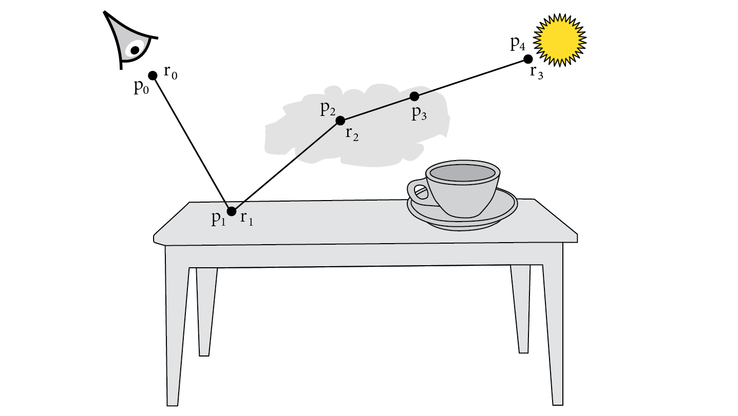
More generally, if there are reflecting or emitting surfaces in the scene, rays do not necessarily have infinite length and the first surface that a ray hits affects its radiance, adding outgoing radiance from the surface at the point and preventing radiance from points along the ray beyond the intersection point from contributing to radiance at the ray’s origin. If a ray ( normal p Subscript , omega Subscript ) intersects a surface at some point normal p Subscript normal s at a parametric distance t along the ray, then the integral equation of transfer is

upper L Subscript normal i Baseline left-parenthesis normal p Subscript Baseline comma omega Subscript Baseline right-parenthesis equals upper T Subscript normal r Baseline left-parenthesis normal p Subscript normal s Baseline right-arrow normal p Subscript Baseline right-parenthesis upper L Subscript normal o Baseline left-parenthesis normal p Subscript normal s Baseline comma minus omega Subscript Baseline right-parenthesis plus integral Subscript 0 Superscript t Baseline upper T Subscript normal r Baseline left-parenthesis normal p prime right-arrow normal p Subscript Baseline right-parenthesis sigma Subscript normal t Baseline left-parenthesis normal p prime comma omega Subscript Baseline right-parenthesis upper L Subscript normal s Superscript Baseline left-parenthesis normal p prime comma minus omega Subscript Baseline right-parenthesis normal d t Superscript prime Baseline comma

where normal p prime equals normal p Subscript Baseline plus t prime omega Subscript are points along the ray (Figure 14.2).

Figure 14.2: For a finite ray that intersects a surface, the incident radiance, upper L Subscript normal i Baseline left-parenthesis normal p Subscript Baseline comma omega Subscript Baseline right-parenthesis , is equal to the outgoing radiance from the surface, upper L Subscript normal o Superscript Baseline left-parenthesis normal p Subscript normal s Baseline comma minus omega Subscript Baseline right-parenthesis , times the beam transmittance to the surface plus the added radiance from all points along the ray from normal p Subscript to  normal p Subscript normal s .

This equation describes the two effects that contribute to radiance along the ray. First, reflected radiance back along the ray from the surface is given by the upper L Subscript normal o term, which gives the emitted and reflected radiance from the surface. This radiance may be attenuated by the participating media; the beam transmittance from the ray origin to the point normal p Subscript normal s accounts for this. The second term accounts for the added radiance along the ray due to volumetric scattering and emission up to the point where the ray intersects the surface; points beyond that one do not affect the radiance along the ray.

14.1.1 Null-Scattering Extension

In Section 11.2.1 we saw the value of null scattering, which made it possible to sample from a modified transmittance equation and to compute unbiased estimates of the transmittance between two points using algorithms like delta tracking and ratio tracking. Null scattering can be applied in a similar way to the equation of transfer, giving similar benefits.

In order to simplify notation in the following, we will assume that the various scattering coefficients sigma do not vary as a function of direction. As before, we will also assume that the null-scattering coefficient sigma Subscript normal n is nonnegative and has been set to homogenize the medium’s density to a fixed majorant sigma Subscript normal m normal a normal j Baseline equals sigma Subscript normal n Baseline plus sigma Subscript normal t . Neither of these simplifications affect the course of the following derivations; both generalizations could be easily reintroduced.

A null-scattering generalization of the equation of transfer can be found using the relationship sigma Subscript normal t Baseline equals sigma Subscript normal m normal a normal j Baseline minus sigma Subscript normal n from Equation (11.11). If that substitution is made in the integro-differential equation of transfer, Equation (14.1), and the boundary condition of a surface at distance t along the ray is applied, then the result can be transformed into the pure integral equation

StartLayout 1st Row 1st Column upper L Subscript normal i Baseline left-parenthesis normal p Subscript Baseline comma omega Subscript Baseline right-parenthesis equals 2nd Column upper T Subscript normal m normal a normal j Baseline left-parenthesis normal p Subscript normal s Baseline right-arrow normal p Subscript Baseline right-parenthesis upper L Subscript normal o Baseline left-parenthesis normal p Subscript normal s Baseline comma minus omega Subscript Baseline right-parenthesis 2nd Row 1st Column Blank 2nd Column plus sigma Subscript normal m normal a normal j Baseline integral Subscript 0 Superscript t Baseline upper T Subscript normal m normal a normal j Baseline left-parenthesis normal p prime right-arrow normal p Subscript Baseline right-parenthesis upper L Subscript normal n Baseline left-parenthesis normal p prime comma minus omega Subscript Baseline right-parenthesis normal d t Superscript prime Baseline comma EndLayout

where normal p prime equals normal p Subscript Baseline plus t prime omega Subscript , as before, and we have introduced upper T Subscript normal m normal a normal j to denote the majorant transmittance that accounts for both regular attenuation and null scattering. Using the same convention as before that d equals double-vertical-bar normal p Subscript Baseline minus normal p prime double-vertical-bar is the distance between points normal p Subscript and normal p prime , it is

upper T Subscript normal m normal a normal j Baseline left-parenthesis normal p prime right-arrow normal p Subscript Baseline right-parenthesis equals normal e Superscript integral Subscript 0 Superscript d Baseline minus left-parenthesis sigma Super Subscript normal t Superscript left-parenthesis normal p Super Subscript Superscript plus t omega Super Subscript Superscript right-parenthesis plus sigma Super Subscript normal n Superscript left-parenthesis normal p Super Subscript Superscript plus t omega Super Subscript Superscript right-parenthesis right-parenthesis normal d t Baseline equals normal e Superscript minus sigma Super Subscript normal m normal a normal j Superscript d Baseline period

The null-scattering source function upper L Subscript normal n is the source function upper L Subscript normal s from Equation (11.3) plus a new third term:

StartLayout 1st Row 1st Column upper L Subscript normal n Baseline left-parenthesis normal p Subscript Baseline comma omega Subscript Baseline right-parenthesis equals 2nd Column StartFraction sigma Subscript normal a Baseline left-parenthesis normal p Subscript Baseline right-parenthesis Over sigma Subscript normal m normal a normal j Baseline EndFraction upper L Subscript normal e Baseline left-parenthesis normal p Subscript Baseline comma omega Subscript Baseline right-parenthesis plus StartFraction sigma Subscript normal s Baseline left-parenthesis normal p Subscript Baseline right-parenthesis Over sigma Subscript normal m normal a normal j Baseline EndFraction integral Underscript script upper S squared Endscripts p left-parenthesis normal p Subscript Baseline comma omega Subscript normal i Baseline comma omega Subscript Baseline right-parenthesis upper L Subscript normal i Baseline left-parenthesis normal p Subscript Baseline comma omega Subscript normal i Baseline right-parenthesis normal d omega Subscript normal i 2nd Row 1st Column Blank 2nd Column plus StartFraction sigma Subscript normal n Baseline left-parenthesis normal p Subscript Baseline right-parenthesis Over sigma Subscript normal m normal a normal j Baseline EndFraction upper L Subscript normal i Baseline left-parenthesis normal p Subscript Baseline comma omega Subscript Baseline right-parenthesis period EndLayout

Because it includes attenuation due to null scattering, upper T Subscript normal m normal a normal j is always less than or equal to the actual transmittance. Thus, the product upper T Subscript normal m normal a normal j Baseline upper L Subscript normal o in Equation (14.3) may be less than the actual contribution of radiance leaving the surface, upper T Subscript normal r Baseline upper L Subscript normal o . However, any such deficiency is made up for by the last term of Equation (14.5).

14.1.2 Evaluating the Equation of Transfer

The upper T Subscript normal m normal a normal j factor in the null-scattering equation of transfer gives a convenient distribution for sampling distances t along the ray in the medium that leads to the volumetric path-tracing algorithm, which we will now describe. (The algorithm we will arrive at is sometimes described as using delta tracking to solve the equation of transfer, since that is the sampling technique it uses for finding the locations of absorption and scattering events.)

If we assume for now that there is no geometry in the scene, then the null-scattering equation of transfer, Equation (14.3), simplifies to

upper L Subscript normal i Baseline left-parenthesis normal p Subscript Baseline comma omega Subscript Baseline right-parenthesis equals sigma Subscript normal m normal a normal j Baseline integral Subscript 0 Superscript normal infinity Baseline upper T Subscript normal m normal a normal j Baseline left-parenthesis normal p prime right-arrow normal p Subscript Baseline right-parenthesis upper L Subscript normal n Baseline left-parenthesis normal p prime comma minus omega Subscript Baseline right-parenthesis normal d t Superscript prime Baseline period

Thanks to null scattering having made the majorant medium homogeneous, sigma Subscript normal m normal a normal j Baseline upper T Subscript normal m normal a normal j can be sampled exactly. The first step in the path-tracing algorithm is to sample a point normal p prime from its distribution, giving the estimator

upper L Subscript normal i Baseline left-parenthesis normal p Subscript Baseline comma omega Subscript Baseline right-parenthesis almost-equals StartFraction sigma Subscript normal m normal a normal j Baseline upper T Subscript normal m normal a normal j Baseline left-parenthesis normal p prime right-arrow normal p Subscript Baseline right-parenthesis upper L Subscript normal n Baseline left-parenthesis normal p prime comma minus omega Subscript Baseline right-parenthesis Over p left-parenthesis normal p Superscript prime Baseline right-parenthesis EndFraction period

From Section A.4.2, we know that the probability density function (PDF) for sampling a distance t from the exponential distribution normal e Superscript minus sigma Super Subscript normal m normal a normal j Superscript t is p left-parenthesis t right-parenthesis equals sigma Subscript normal m normal a normal j Baseline normal e Superscript minus sigma Super Subscript normal m normal a normal j Superscript t , and so the estimator simplifies to

upper L Subscript normal i Baseline left-parenthesis normal p Subscript Baseline comma omega Subscript Baseline right-parenthesis almost-equals upper L Subscript normal n Baseline left-parenthesis normal p prime comma minus omega Subscript Baseline right-parenthesis period

What is left is to evaluate upper L Subscript normal n .

Because sigma Subscript normal m normal a normal j Baseline equals sigma Subscript normal a Baseline plus sigma Subscript normal s Baseline plus sigma Subscript normal n , the initial sigma factors in each term of Equation (14.5) can be considered to be three probabilities that sum to 1. If one of the three terms is randomly selected according to its probability and the rest of the term is evaluated without that factor, the expected value of the result is equal to upper L Subscript normal n . Considering how to evaluate each of the terms:

  • If the sigma Subscript normal a term is chosen, then the emission at upper L Subscript normal e Baseline left-parenthesis normal p prime comma omega Subscript Baseline right-parenthesis is returned and sampling terminates.
  • For the sigma Subscript normal s term, the integral over the sphere of directions must be estimated. A direction omega prime Subscript is sampled from some distribution and recursive evaluation of upper L Subscript normal i Baseline left-parenthesis normal p prime comma omega prime Subscript Baseline right-parenthesis then proceeds, weighted by the ratio of the phase function and the probability of sampling the direction omega prime Subscript .
  • If the null-scattering term is selected, upper L Subscript normal i Baseline left-parenthesis normal p prime comma omega Subscript Baseline right-parenthesis is to be evaluated, which can be handled recursively as well.

For the full equation of transfer that includes scattering from surfaces, both the surface-scattering term and the integral over the ray’s extent lead to recursive evaluation of the equation of transfer. In the context of path tracing, however, we would like to only evaluate one of the terms in order to avoid an exponential increase in work. We will therefore start by defining a probability q of estimating the surface-scattering term; volumetric scattering is evaluated otherwise. Given such a q , the Monte Carlo estimator

upper L Subscript normal i Baseline left-parenthesis normal p Subscript Baseline comma omega Subscript Baseline right-parenthesis almost-equals StartLayout Enlarged left-brace 1st Row 1st Column StartFraction upper T Subscript normal m normal a normal j Baseline left-parenthesis normal p Subscript normal s Baseline right-arrow normal p Subscript Baseline right-parenthesis upper L Subscript normal o Baseline left-parenthesis normal p Subscript normal s Baseline comma minus omega Subscript Baseline right-parenthesis Over q EndFraction comma 2nd Column with probability q 2nd Row 1st Column StartFraction sigma Subscript normal m normal a normal j Baseline integral Subscript 0 Superscript t Baseline upper T Subscript normal m normal a normal j Baseline left-parenthesis normal p prime right-arrow normal p Subscript Baseline right-parenthesis upper L Subscript normal n Baseline left-parenthesis normal p prime comma minus omega Subscript Baseline right-parenthesis normal d t Superscript prime Baseline Over 1 minus q EndFraction comma 2nd Column otherwise EndLayout

gives upper L Subscript normal i Baseline left-parenthesis normal p Subscript Baseline comma omega Subscript Baseline right-parenthesis in expectation.

A good choice for q is that it be equal to upper T Subscript normal m normal a normal j Baseline left-parenthesis normal p Subscript normal s Baseline right-arrow normal p Subscript Baseline right-parenthesis . Surface scattering is then evaluated with a probability proportional to the transmittance to the surface and the ratio upper T Subscript normal m normal a normal j Baseline slash q is equal to 1, leaving just the upper L Subscript normal o factor. Furthermore, a sampling trick can be used to choose between the two terms: if a sample t prime element-of left-bracket 0 comma normal infinity right-parenthesis is taken from sigma Subscript normal m normal a normal j Baseline upper T Subscript normal m normal a normal j ’s distribution, then the probability that t prime greater-than t is equal to upper T Subscript normal m normal a normal j Baseline left-parenthesis normal p Subscript normal s Baseline right-arrow normal p Subscript Baseline right-parenthesis . (This can be shown by integrating upper T Subscript normal m normal a normal j ’s PDF to find its cumulative distribution function (CDF) and then considering the value of its CDF at t .) Using this technique and then making the same simplifications that brought us to Equation (14.6), we arrive at the estimator

upper L Subscript normal i Baseline left-parenthesis normal p Subscript Baseline comma omega Subscript Baseline right-parenthesis almost-equals StartLayout Enlarged left-brace 1st Row 1st Column upper L Subscript normal o Baseline left-parenthesis normal p Subscript normal s Baseline comma omega Subscript Baseline right-parenthesis comma 2nd Column if t prime greater-than t 2nd Row 1st Column upper L Subscript normal n Baseline left-parenthesis normal p prime comma minus omega Subscript Baseline right-parenthesis comma 2nd Column otherwise period EndLayout

From this point, outgoing radiance from a surface can be estimated using techniques that were introduced in Chapter 13, and upper L Subscript normal n can be estimated as described earlier.

14.1.3 Sampling the Majorant Transmittance

We have so far presented volumetric path tracing with the assumption that sigma Subscript normal m normal a normal j is constant along the ray and thus that upper T Subscript normal m normal a normal j is a single exponential function. However, those assumptions are not compatible with the segments of piecewise-constant majorants that Medium implementations provide with their RayMajorantIterators. We will now resolve this incompatibility.

Figure 14.3: (a) Given piecewise-constant majorants defined over segments along a ray, the corresponding optical thickness tau is a piecewise-linear function. (b) Exponentiating the negative optical thickness gives the transmittance at each point along the ray. The transmittance function is continuous and decreasing, but has a first derivative discontinuity at transitions between segments.

Figure 14.3 shows example majorants along a ray, the optical thickness that they integrate to, and the resulting majorant transmittance function. The transmittance function is continuous and strictly decreasing, though at a rate that depends on the majorant at each point along the ray. If integration starts from t equals 0 , and we denote the i th segment’s majorant as sigma Subscript normal m normal a normal j Superscript i and its endpoint as normal p Subscript Baseline Subscript i , the transmittance can be written as

upper T Subscript normal m normal a normal j Baseline left-parenthesis normal p Subscript Baseline right-arrow normal p prime right-parenthesis equals upper T Subscript normal m normal a normal j Superscript 1 Baseline left-parenthesis normal p Subscript Baseline right-arrow normal p 1 right-parenthesis upper T Subscript normal m normal a normal j Superscript 2 Baseline left-parenthesis normal p 1 right-arrow normal p 2 right-parenthesis midline-horizontal-ellipsis upper T Subscript normal m normal a normal j Superscript n Baseline left-parenthesis normal p Subscript n minus 1 Baseline right-arrow normal p prime right-parenthesis

where upper T Subscript normal m normal a normal j Superscript i is the transmittance function for the i th segment and the point normal p prime is the endpoint of the n th segment. (This relationship uses the multiplicative property of transmittance from Equation (11.6).)

Given the general task of estimating an integral of the form

integral Subscript 0 Superscript t Baseline sigma Subscript normal m normal a normal j Baseline left-parenthesis normal p prime right-parenthesis upper T Subscript normal m normal a normal j Baseline left-parenthesis normal p Subscript Baseline right-arrow normal p Superscript prime Baseline right-parenthesis f left-parenthesis normal p prime right-parenthesis normal d t prime

with normal p prime equals normal p Subscript Baseline plus t prime omega Subscript and omega Subscript Baseline equals ModifyingAbove normal p prime minus normal p Subscript Baseline With caret , it is useful to rewrite the integral to be over the individual majorant segments, which gives

StartLayout 1st Row 1st Column sigma Subscript normal m normal a normal j Superscript 1 2nd Column integral Subscript 0 Superscript t 1 Baseline upper T Subscript normal m normal a normal j Superscript 1 Baseline left-parenthesis normal p Subscript Baseline right-arrow normal p Superscript prime Baseline right-parenthesis f left-parenthesis normal p prime right-parenthesis normal d t prime 2nd Row 1st Column Blank 2nd Column plus sigma Subscript normal m normal a normal j Superscript 1 Baseline upper T Subscript normal m normal a normal j Superscript 1 Baseline left-parenthesis normal p Subscript Baseline right-arrow normal p 1 right-parenthesis sigma Subscript normal m normal a normal j Superscript 2 Baseline integral Subscript t 1 Superscript t 2 Baseline upper T Subscript normal m normal a normal j Superscript 2 Baseline left-parenthesis normal p 1 right-arrow normal p Superscript prime Baseline right-parenthesis f left-parenthesis normal p prime right-parenthesis normal d t prime 3rd Row 1st Column Blank 2nd Column plus sigma Subscript normal m normal a normal j Superscript 1 Baseline upper T Subscript normal m normal a normal j Superscript 1 Baseline left-parenthesis normal p Subscript Baseline right-arrow normal p 1 right-parenthesis sigma Subscript normal m normal a normal j Superscript 2 Baseline upper T Subscript normal m normal a normal j Superscript 2 Baseline left-parenthesis normal p 1 right-arrow normal p 2 right-parenthesis integral Subscript t 2 Superscript t 3 Baseline upper T Subscript normal m normal a normal j Superscript 3 Baseline left-parenthesis normal p 2 right-arrow normal p Superscript prime Baseline right-parenthesis f left-parenthesis normal p Superscript prime Baseline right-parenthesis normal d t Superscript prime Baseline plus midline-horizontal-ellipsis period EndLayout

Note that each term’s contribution is modulated by the transmittances and majorants from the previous segments.

The form of Equation (14.8) hints at a sampling strategy: we start by sampling a value t prime 1 from upper T Subscript normal m normal a normal j Superscript 1 ’s distribution p 1 ; if t prime 1 is less than t 1 , then we evaluate the estimator at the sampled point  normal p prime :

StartFraction sigma Subscript normal m normal a normal j Superscript 1 Baseline upper T Subscript normal m normal a normal j Superscript 1 Baseline left-parenthesis normal p Subscript Baseline right-arrow normal p Superscript prime Baseline right-parenthesis f left-parenthesis normal p Superscript prime Baseline right-parenthesis Over p 1 left-parenthesis t prime 1 right-parenthesis EndFraction equals f left-parenthesis normal p Superscript prime Baseline right-parenthesis period

Applying the same ideas that led to Equation (14.7), we otherwise continue and consider the second term, drawing a sample t prime 2 from upper T Subscript normal m normal a normal j Superscript 2 ’s distribution, starting at t 1 . If the sampled point is before the segment’s endpoint, t prime 2 less-than t 2 , then we have the estimator

StartFraction sigma Subscript normal m normal a normal j Superscript 1 Baseline upper T Subscript normal m normal a normal j Superscript 1 Baseline left-parenthesis normal p Subscript Baseline right-arrow normal p 1 right-parenthesis sigma Subscript normal m normal a normal j Superscript 2 Baseline upper T Subscript normal m normal a normal j Superscript 2 Baseline left-parenthesis normal p 1 right-arrow normal p Superscript prime Baseline right-parenthesis f left-parenthesis normal p Superscript prime Baseline right-parenthesis Over probability left-brace t prime 1 greater-than t 1 right-brace p 2 left-parenthesis t prime 2 right-parenthesis EndFraction period

Because the probability that t prime 1 greater-than t is equal to sigma Subscript normal m normal a normal j Superscript 1 Baseline upper T Subscript normal m normal a normal j Superscript 1 Baseline left-parenthesis normal p Subscript Baseline right-arrow normal p 1 right-parenthesis , the estimator for the second term again simplifies to f left-parenthesis normal p prime right-parenthesis . Otherwise, following this sampling strategy for subsequent segments similarly leads to the same simplified estimator in the end. It can furthermore be shown that the probability that no sample is generated in any of the segments is equal to the full majorant transmittance from 0 to  t , which is exactly the probability required for the surface/volume estimator of Equation (14.7).

The SampleT_maj() function implements this sampling strategy, handling the details of iterating over RayMajorantSegments and sampling them. Its functionality will be used repeatedly in the following volumetric integrators.

<<Medium Sampling Functions>>= 
template <typename F> SampledSpectrum SampleT_maj(Ray ray, Float tMax, Float u, RNG &rng, const SampledWavelengths &lambda, F callback);

In addition to a ray and an endpoint along it specified by tMax, SampleT_maj() takes a single uniform sample and an RNG to use for generating any necessary additional samples. This allows it to use a well-distributed value from a Sampler for the first sampling decision along the ray while it avoids consuming a variable and unbounded number of sample dimensions if more are needed (recall the discussion of the importance of consistency in sample dimension consumption in Section 8.3).

The provided SampledWavelengths play their usual role, though the first of them has additional meaning: for media with scattering properties that vary with wavelength, the majorant at the first wavelength is used for sampling. The alternative would be to sample each wavelength independently, though that would cause an explosion in samples to be evaluated in the context of algorithms like path tracing. Sampling a single wavelength can work well for evaluating all wavelengths’ contributions if multiple importance sampling (MIS) is used; this topic is discussed further in Section 14.2.2.

A callback function is the last parameter passed to SampleT_maj(). This is a significant difference from pbrt’s other sampling methods, which all generate a single sample (or sometimes, no sample) each time they are called. When sampling media that has null scattering, however, often a succession of samples are needed along the same ray. (Delta tracking, described in Section 11.2.1, is an example of such an algorithm.) The provided callback function is therefore invoked by SampleT_maj() each time a sample is taken. After the callback processes the sample, it should return a Boolean value that indicates whether sampling should recommence starting from the provided sample. With this implementation approach, SampleT_maj() can maintain state like the RayMajorantIterator between samples along a ray, which improves efficiency.

The signature of the callback function should be the following:

bool callback(Point3f p, MediumProperties mp, SampledSpectrum sigma_maj, SampledSpectrum T_maj)

Each invocation of the callback is passed a sampled point along the ray, the associated MediumProperties and sigma Subscript normal m normal a normal j for the medium at that point, and the majorant transmittance upper T Subscript normal m normal a normal j . The first time callback is invoked, the majorant transmittance will be from the ray origin to the sample; any subsequent invocations give the transmittance from the previous sample to the current one.

After sampling concludes, SampleT_maj() returns the majorant transmittance upper T Subscript normal m normal a normal j from the last sampled point in the medium (or the ray origin, if no samples were generated) to the ray’s endpoint (see Figure 14.4).

Figure 14.4: In addition to calling a provided callback function at sampled points in the medium, shown here as filled circles, the SampleT_maj() function returns the majorant transmittance upper T Subscript normal m normal a normal j from the last sampled point to the provided t Subscript normal m normal a normal x value.

As if all of this was not sufficiently complex, the implementation of SampleT_maj() starts out with some tricky C++ code. There is a second variant of SampleT_maj() we will introduce shortly that is templated based on the concrete type of Medium being sampled. In order to call the appropriate template specialization, we must determine which type of Medium the ray is passing through. Conceptually, we would like to do something like the following, using the TaggedPointer::Is() method:

if (ray.medium.Is<HomogeneousMedium>()) SampleT_maj<HomogeneousMedium>(ray, tMax, u,rng, lambda, func); else if (ray.medium.Is<UniformGridMedium>()) // …

However, enumerating all the media that are implemented in pbrt in the SampleT_maj() function is undesirable: that would add an unexpected and puzzling additional step for users who wanted to extend the system with a new Medium. Therefore, the first SampleT_maj() function uses the dynamic dispatch capability of the Medium’s TaggedPointer along with a generic lambda function, sample, to determine the Medium’s type. TaggedPointer::Dispatch() ends up passing the Medium pointer back to sample; because the parameter is declared as auto, it then takes on the actual type of the medium when it is invoked. Thus, the following function has equivalent functionality to the code above but naturally handles all the media that are listed in the Medium class declaration without further modification.

<<Medium Sampling Function Definitions>>+=  
template <typename F> SampledSpectrum SampleT_maj(Ray ray, Float tMax, Float u, RNG &rng, const SampledWavelengths &lambda, F callback) { auto sample = [&](auto medium) { using M = typename std::remove_reference_t<decltype(*medium)>; return SampleT_maj<M>(ray, tMax, u, rng, lambda, callback); }; return ray.medium.Dispatch(sample); }

With the concrete type of the medium available, we can proceed with the second instance of SampleTmaj(), which can now be specialized based on that type.

<<Medium Sampling Function Definitions>>+= 
template <typename ConcreteMedium, typename F> SampledSpectrum SampleT_maj(Ray ray, Float tMax, Float u, RNG &rng, const SampledWavelengths &lambda, F callback) { <<Normalize ray direction and update tMax accordingly>> 
tMax *= Length(ray.d); ray.d = Normalize(ray.d);
<<Initialize MajorantIterator for ray majorant sampling>> 
ConcreteMedium *medium = ray.medium.Cast<ConcreteMedium>(); typename ConcreteMedium::MajorantIterator iter = medium->SampleRay(ray, tMax, lambda);
<<Generate ray majorant samples until termination>> 
SampledSpectrum T_maj(1.f); bool done = false; while (!done) { <<Get next majorant segment from iterator and sample it>> 
pstd::optional<RayMajorantSegment> seg = iter.Next(); if (!seg) return T_maj; <<Handle zero-valued majorant for current segment>> 
if (seg->sigma_maj[0] == 0) { Float dt = seg->tMax - seg->tMin; <<Handle infinite dt for ray majorant segment>> 
if (IsInf(dt)) dt = std::numeric_limits<Float>::max();
T_maj *= FastExp(-dt * seg->sigma_maj); continue; }
<<Generate samples along current majorant segment>> 
Float tMin = seg->tMin; while (true) { <<Try to generate sample along current majorant segment>> 
Float t = tMin + SampleExponential(u, seg->sigma_maj[0]); u = rng.Uniform<Float>(); if (t < seg->tMax) { <<Call callback function for sample within segment>> 
T_maj *= FastExp(-(t - tMin) * seg->sigma_maj); MediumProperties mp = medium->SamplePoint(ray(t), lambda); if (!callback(ray(t), mp, seg->sigma_maj, T_maj)) { done = true; break; } T_maj = SampledSpectrum(1.f); tMin = t;
} else { <<Handle sample past end of majorant segment>> 
Float dt = seg->tMax - tMin; T_maj *= FastExp(-dt * seg->sigma_maj); break;
}
}
} return SampledSpectrum(1.f);
}

The function starts by normalizing the ray’s direction so that parametric distance along the ray directly corresponds to distance from the ray’s origin. This simplifies subsequent transmittance computations in the remainder of the function. Since normalization scales the direction’s length, the tMax endpoint must also be updated so that it corresponds to the same point along the ray.

<<Normalize ray direction and update tMax accordingly>>= 
tMax *= Length(ray.d); ray.d = Normalize(ray.d);

Since the actual type of the medium is known and because all Medium implementations must define a MajorantIterator type (recall Section 11.4.1), the medium’s iterator type can be directly declared as a stack-allocated variable. This gives a number of benefits: not only is the expense of dynamic allocation avoided, but subsequent calls to the iterator’s Next() method in this function are regular method calls that can even be expanded inline by the compiler; no dynamic dispatch is necessary for them. An additional benefit of knowing the medium’s type is that the appropriate SampleRay() method can be called directly without incurring the cost of dynamic dispatch here.

<<Initialize MajorantIterator for ray majorant sampling>>= 
ConcreteMedium *medium = ray.medium.Cast<ConcreteMedium>(); typename ConcreteMedium::MajorantIterator iter = medium->SampleRay(ray, tMax, lambda);

With an iterator initialized, sampling along the ray can proceed. The T_maj variable declared here tracks the accumulated majorant transmittance from the ray origin or the previous sample along the ray (depending on whether a sample has yet been generated).

<<Generate ray majorant samples until termination>>= 
SampledSpectrum T_maj(1.f); bool done = false; while (!done) { <<Get next majorant segment from iterator and sample it>> 
pstd::optional<RayMajorantSegment> seg = iter.Next(); if (!seg) return T_maj; <<Handle zero-valued majorant for current segment>> 
if (seg->sigma_maj[0] == 0) { Float dt = seg->tMax - seg->tMin; <<Handle infinite dt for ray majorant segment>> 
if (IsInf(dt)) dt = std::numeric_limits<Float>::max();
T_maj *= FastExp(-dt * seg->sigma_maj); continue; }
<<Generate samples along current majorant segment>> 
Float tMin = seg->tMin; while (true) { <<Try to generate sample along current majorant segment>> 
Float t = tMin + SampleExponential(u, seg->sigma_maj[0]); u = rng.Uniform<Float>(); if (t < seg->tMax) { <<Call callback function for sample within segment>> 
T_maj *= FastExp(-(t - tMin) * seg->sigma_maj); MediumProperties mp = medium->SamplePoint(ray(t), lambda); if (!callback(ray(t), mp, seg->sigma_maj, T_maj)) { done = true; break; } T_maj = SampledSpectrum(1.f); tMin = t;
} else { <<Handle sample past end of majorant segment>> 
Float dt = seg->tMax - tMin; T_maj *= FastExp(-dt * seg->sigma_maj); break;
}
}
} return SampledSpectrum(1.f);

If the iterator has no further majorant segments to provide, then sampling is complete. In this case, it is important to return any majorant transmittance that has accumulated in T_maj; that represents the remaining transmittance to the ray’s endpoint. Otherwise, a few details are attended to before sampling proceeds along the segment.

<<Get next majorant segment from iterator and sample it>>= 
pstd::optional<RayMajorantSegment> seg = iter.Next(); if (!seg) return T_maj; <<Handle zero-valued majorant for current segment>> 
if (seg->sigma_maj[0] == 0) { Float dt = seg->tMax - seg->tMin; <<Handle infinite dt for ray majorant segment>> 
if (IsInf(dt)) dt = std::numeric_limits<Float>::max();
T_maj *= FastExp(-dt * seg->sigma_maj); continue; }
<<Generate samples along current majorant segment>> 
Float tMin = seg->tMin; while (true) { <<Try to generate sample along current majorant segment>> 
Float t = tMin + SampleExponential(u, seg->sigma_maj[0]); u = rng.Uniform<Float>(); if (t < seg->tMax) { <<Call callback function for sample within segment>> 
T_maj *= FastExp(-(t - tMin) * seg->sigma_maj); MediumProperties mp = medium->SamplePoint(ray(t), lambda); if (!callback(ray(t), mp, seg->sigma_maj, T_maj)) { done = true; break; } T_maj = SampledSpectrum(1.f); tMin = t;
} else { <<Handle sample past end of majorant segment>> 
Float dt = seg->tMax - tMin; T_maj *= FastExp(-dt * seg->sigma_maj); break;
}
}

If the majorant has the value 0 in the first wavelength, then there is nothing to sample along the segment. It is important to handle this case, since otherwise the subsequent call to SampleExponential() in this function would return an infinite value that would subsequently lead to not-a-number values. Because the other wavelengths may not themselves have zero-valued majorants, we must still update T_maj for the segment’s majorant transmittance even though the transmittance for the first wavelength is unchanged.

<<Handle zero-valued majorant for current segment>>= 
if (seg->sigma_maj[0] == 0) { Float dt = seg->tMax - seg->tMin; <<Handle infinite dt for ray majorant segment>> 
if (IsInf(dt)) dt = std::numeric_limits<Float>::max();
T_maj *= FastExp(-dt * seg->sigma_maj); continue; }

One edge case must be attended to before the exponential function is called. If tMax holds the IEEE floating-point infinity value, then dt will as well; it then must be bumped down to the largest finite Float. This is necessary because with floating-point arithmetic, zero times infinity gives a not-a-number value (whereas any nonzero value times infinity gives infinity). Otherwise, for any wavelengths with zero-valued sigma_maj, not-a-number values would be passed to FastExp().

<<Handle infinite dt for ray majorant segment>>= 
if (IsInf(dt)) dt = std::numeric_limits<Float>::max();

The implementation otherwise tries to generate a sample along the current segment. This work is inside a while loop so that multiple samples may be generated along the segment.

<<Generate samples along current majorant segment>>= 
Float tMin = seg->tMin; while (true) { <<Try to generate sample along current majorant segment>> 
Float t = tMin + SampleExponential(u, seg->sigma_maj[0]); u = rng.Uniform<Float>(); if (t < seg->tMax) { <<Call callback function for sample within segment>> 
T_maj *= FastExp(-(t - tMin) * seg->sigma_maj); MediumProperties mp = medium->SamplePoint(ray(t), lambda); if (!callback(ray(t), mp, seg->sigma_maj, T_maj)) { done = true; break; } T_maj = SampledSpectrum(1.f); tMin = t;
} else { <<Handle sample past end of majorant segment>> 
Float dt = seg->tMax - tMin; T_maj *= FastExp(-dt * seg->sigma_maj); break;
}
}

In the usual case, a distance is sampled according to the PDF sigma Subscript normal m normal a normal j Baseline normal e Superscript minus sigma Super Subscript normal m normal a normal j Superscript t . Separate cases handle a sample that is within the current majorant segment and one that is past it.

One detail to note in this fragment is that as soon as the uniform sample u has been used, a replacement is immediately generated using the provided RNG. In this way, the method maintains the invariant that u is always a valid independent sample value. While this can lead to a single excess call to RNG::Uniform() each time SampleT_maj() is called, it ensures the initial u value provided to the method is used only once.

<<Try to generate sample along current majorant segment>>= 
Float t = tMin + SampleExponential(u, seg->sigma_maj[0]); u = rng.Uniform<Float>(); if (t < seg->tMax) { <<Call callback function for sample within segment>> 
T_maj *= FastExp(-(t - tMin) * seg->sigma_maj); MediumProperties mp = medium->SamplePoint(ray(t), lambda); if (!callback(ray(t), mp, seg->sigma_maj, T_maj)) { done = true; break; } T_maj = SampledSpectrum(1.f); tMin = t;
} else { <<Handle sample past end of majorant segment>> 
Float dt = seg->tMax - tMin; T_maj *= FastExp(-dt * seg->sigma_maj); break;
}

For a sample within the segment’s extent, the final majorant transmittance to be passed to the callback is found by accumulating the transmittance from tMin to the sample point. The rest of the necessary medium properties can be found using SamplePoint(). If the callback function returns false to indicate that sampling should conclude, then we have a doubly nested while loop to break out of; a break statement takes care of the inner one, and setting done to true causes the outer one to terminate.

If true is returned by the callback, indicating that sampling should restart at the sample that was just generated, then the accumulated transmittance is reset to 1 and tMin is updated to be at the just-taken sample’s position.

<<Call callback function for sample within segment>>= 
T_maj *= FastExp(-(t - tMin) * seg->sigma_maj); MediumProperties mp = medium->SamplePoint(ray(t), lambda); if (!callback(ray(t), mp, seg->sigma_maj, T_maj)) { done = true; break; } T_maj = SampledSpectrum(1.f); tMin = t;

If the sampled distance t is past the end of the segment, then there is no medium interaction along it and it is on to the next segment, if any. In this case, majorant transmittance up to the end of the segment must be accumulated into T_maj so that the complete majorant transmittance along the ray is provided with the next valid sample (if any).

<<Handle sample past end of majorant segment>>= 
Float dt = seg->tMax - tMin; T_maj *= FastExp(-dt * seg->sigma_maj); break;

14.1.4 Generalized Path Space

Just as it was helpful to express the light transport equation (LTE) as a sum over paths of scattering events, it is also helpful to express the null-scattering integral equation of transfer in this form. Doing so makes it possible to apply variance reduction techniques like multiple importance sampling and is a prerequisite for constructing participating medium-aware bidirectional integrators.

Recall how, in Section 13.1.4, the surface form of the LTE was repeatedly substituted into itself to derive the path space contribution function for a path of length n

upper P left-parenthesis normal p Subscript Baseline overbar Subscript n Baseline right-parenthesis equals ModifyingBelow integral Underscript upper A Endscripts integral Underscript upper A Endscripts midline-horizontal-ellipsis integral Underscript upper A Endscripts With bottom-brace Underscript n minus 1 Endscripts upper L Subscript normal e Baseline left-parenthesis normal p Subscript Baseline Subscript n Baseline right-arrow normal p Subscript Baseline Subscript n minus 1 Baseline right-parenthesis upper T left-parenthesis normal p Subscript Baseline overbar Subscript n Baseline right-parenthesis normal d upper A Subscript Baseline left-parenthesis normal p 2 right-parenthesis midline-horizontal-ellipsis normal d upper A Subscript Baseline left-parenthesis normal p Subscript Baseline Subscript n Baseline right-parenthesis comma

where the throughput upper T left-parenthesis normal p Subscript Baseline overbar Subscript n Baseline right-parenthesis was defined as

upper T left-parenthesis normal p Subscript Baseline overbar Subscript n Baseline right-parenthesis equals product Underscript i equals 1 Overscript n minus 1 Endscripts f Subscript Baseline left-parenthesis normal p Subscript Baseline Subscript i plus 1 Baseline right-arrow normal p Subscript Baseline Subscript i Baseline right-arrow normal p Subscript Baseline Subscript i minus 1 Baseline right-parenthesis upper G left-parenthesis normal p Subscript Baseline Subscript i plus 1 Baseline left-right-arrow normal p Subscript Baseline Subscript i Baseline right-parenthesis period

This previous definition only works for surfaces, but using a similar approach of substituting the integral equation of transfer, a medium-aware path integral can be derived. The derivation is laborious and we will just present the final result here. (The “Further Reading” section has a pointer to the full derivation.)

Previously, integration occurred over a Cartesian product of surface locations upper A Superscript n . Now, we will need a formal way of writing down an integral over an arbitrary sequence of each of 2D surface locations upper A , 3D positions in a participating medium upper V where actual scattering occurs, and 3D positions in a participating medium upper V Subscript normal empty-set where null scattering occurs. (The two media upper V and upper V Subscript normal empty-set represent the same volume of space with the same scattering properties, but we will find it handy to distinguish between them in the following.)

First, we will focus only on a specific arrangement of n surface and medium vertices encoded in a configuration vector bold c . The associated set of paths is given by a Cartesian product of surface locations and medium locations,

script upper P Subscript n Superscript bold c Baseline equals times Underscript i equals 1 Overscript n Endscripts StartLayout Enlarged left-brace 1st Row 1st Column upper A comma 2nd Column if bold c Subscript i Baseline equals 0 2nd Row 1st Column upper V comma 2nd Column if bold c Subscript i Baseline equals 1 3rd Row 1st Column upper V Subscript normal empty-set Baseline comma 2nd Column if bold c Subscript i Baseline equals 2 period EndLayout

The set of all paths of length n is the union of the above sets over all possible configuration vectors:

script upper P Subscript n Baseline equals union Underscript bold c element-of left-brace 0 comma 1 comma 2 right-brace Superscript n Baseline Endscripts script upper P Subscript n Superscript bold c Baseline period

Next, we define a measure, which provides an abstract notion of the volume of a subset upper D subset-of-or-equal-to script upper P Subscript n that is essential for integration. The measure we will use simply sums up the product of surface area and volume associated with the individual vertices in each of the path spaces of specific configurations.

mu Subscript n Baseline left-parenthesis upper D right-parenthesis equals sigma-summation Underscript bold c element-of left-brace 0 comma 1 right-brace Superscript n Baseline Endscripts mu Subscript n Superscript bold c Baseline left-parenthesis upper D intersection script upper P Subscript n Superscript bold c Baseline right-parenthesis where mu Subscript n Superscript bold c Baseline left-parenthesis upper D right-parenthesis equals integral Underscript upper D Endscripts product Underscript i equals 1 Overscript n Endscripts StartLayout Enlarged left-brace 1st Row 1st Column normal d upper A left-parenthesis normal p Subscript i Baseline right-parenthesis comma 2nd Column if bold c Subscript i Baseline equals 0 2nd Row 1st Column normal d upper V left-parenthesis normal p Subscript i Baseline right-parenthesis comma 2nd Column if bold c Subscript i Baseline equals 1 3rd Row 1st Column normal d upper V Subscript normal empty-set Baseline left-parenthesis normal p Subscript i Baseline right-parenthesis comma 2nd Column if bold c Subscript i Baseline equals 2 period EndLayout

The measure for null-scattering vertices normal d upper V Subscript normal empty-set incorporates a Dirac delta distribution to limit integration to be along the line between successive real-scattering vertices.

The generalized path contribution ModifyingAbove upper P With caret left-parenthesis normal p Subscript Baseline overbar Subscript n Baseline right-parenthesis can now be written as

ModifyingAbove upper P With caret left-parenthesis normal p Subscript Baseline overbar Subscript n Baseline right-parenthesis equals integral Underscript script upper P Subscript n minus 1 Baseline Endscripts ModifyingAbove upper L With caret Subscript normal e Baseline left-parenthesis normal p Subscript Baseline Subscript n Baseline right-arrow normal p Subscript Baseline Subscript n minus 1 Baseline right-parenthesis ModifyingAbove upper T With caret left-parenthesis normal p Subscript Baseline overbar Subscript n Baseline right-parenthesis normal d mu Subscript n minus 1 Baseline left-parenthesis normal p 2 comma ellipsis comma normal p Subscript n Baseline right-parenthesis comma

where

ModifyingAbove upper L With caret Subscript normal e Baseline left-parenthesis normal p Subscript Baseline Subscript n Baseline right-arrow normal p Subscript Baseline Subscript n minus 1 Baseline right-parenthesis equals StartLayout Enlarged left-brace 1st Row 1st Column upper L Subscript normal e Baseline left-parenthesis normal p Subscript Baseline Subscript n Baseline right-arrow normal p Subscript Baseline Subscript n minus 1 Baseline right-parenthesis 2nd Column if normal p Subscript Baseline Subscript n Baseline element-of upper A comma 2nd Row 1st Column sigma Subscript normal a Baseline left-parenthesis normal p Subscript Baseline Subscript n Baseline right-parenthesis upper L Subscript normal e Baseline left-parenthesis normal p Subscript Baseline Subscript n Baseline right-arrow normal p Subscript Baseline Subscript n minus 1 Baseline right-parenthesis 2nd Column if normal p Subscript Baseline Subscript n Baseline element-of upper V period EndLayout

Due to the measure defined earlier, the generalized path contribution is a sum of many integrals considering all possible sequences of surface, volume, and null-scattering events.

The full set of path vertices normal p Subscript Baseline Subscript i include both null- and real-scattering events. We will find it useful to use normal r Subscript i to denote the subset of them that represent real scattering (see Figure 14.5). Note a given real-scattering vertex normal r Subscript i will generally have a different index value in the full path.

Figure 14.5: In the path space framework, a path is defined by a set of n vertices normal p Subscript Baseline Subscript i that have an emitter at one endpoint and a sensor at the other, where intermediate vertices represent scattering events, including null scattering. The subset of m vertices that represent real scattering events are labeled normal r Subscript i .

The path throughput function ModifyingAbove upper T With caret left-parenthesis normal p Subscript Baseline overbar Subscript n Baseline right-parenthesis can then be defined as:

StartLayout 1st Row 1st Column ModifyingAbove upper T With caret left-parenthesis normal p Subscript Baseline overbar Subscript n Baseline right-parenthesis equals 2nd Column left-parenthesis product Underscript i equals 1 Overscript n minus 1 Endscripts ModifyingAbove f With caret left-parenthesis normal p Subscript Baseline Subscript i plus 1 Baseline right-arrow normal p Subscript Baseline Subscript i Baseline right-arrow normal p Subscript Baseline Subscript i minus 1 Baseline right-parenthesis right-parenthesis left-parenthesis product Underscript i equals 0 Overscript n minus 1 Endscripts upper T Subscript normal m normal a normal j Baseline left-parenthesis normal p Subscript Baseline Subscript i Baseline right-arrow normal p Subscript Baseline Subscript i plus 1 Baseline right-parenthesis right-parenthesis 2nd Row 1st Column Blank 2nd Column times left-parenthesis product Underscript i equals 1 Overscript m minus 1 Endscripts ModifyingAbove upper G With caret left-parenthesis normal r Subscript i Baseline left-right-arrow normal r Subscript i plus 1 Baseline right-parenthesis right-parenthesis EndLayout

It now refers to a generalized scattering distribution function ModifyingAbove f With caret and generalized geometric term ModifyingAbove upper G With caret . The former simply falls back to the BSDF, phase function (multiplied by sigma Subscript normal s ), or a factor that enforces the ordering of null-scattering vertices, depending on the type of the vertex normal p Subscript i . Note that the first two products in Equation (14.11) are over all vertices but the third is only over real-scattering vertices.

The scattering distribution function ModifyingAbove f With caret is defined by

ModifyingAbove f With caret left-parenthesis normal p Subscript Baseline Subscript i plus 1 Baseline right-arrow normal p Subscript Baseline Subscript i Baseline right-arrow normal p Subscript Baseline Subscript i minus 1 Baseline right-parenthesis equals StartLayout Enlarged left-brace 1st Row 1st Column f Subscript Baseline left-parenthesis normal p Subscript Baseline Subscript i plus 1 Baseline right-arrow normal p Subscript Baseline Subscript i Baseline right-arrow normal p Subscript Baseline Subscript i minus 1 Baseline right-parenthesis comma 2nd Column if normal p Subscript Baseline Subscript i Baseline element-of upper A 2nd Row 1st Column sigma Subscript normal s Baseline left-parenthesis normal p Subscript Baseline Subscript i Baseline right-parenthesis p Subscript Baseline left-parenthesis normal p Subscript Baseline Subscript i plus 1 Baseline right-arrow normal p Subscript Baseline Subscript i Baseline right-arrow normal p Subscript Baseline Subscript i minus 1 Baseline right-parenthesis comma 2nd Column if normal p Subscript Baseline Subscript i Baseline element-of upper V 3rd Row 1st Column sigma Subscript normal n Baseline left-parenthesis normal p Subscript Baseline Subscript i Baseline right-parenthesis upper H left-parenthesis left-parenthesis normal p Subscript Baseline Subscript i Baseline minus normal p Subscript Baseline Subscript i plus 1 Baseline right-parenthesis dot left-parenthesis normal p Subscript Baseline Subscript i minus 1 Baseline minus normal p Subscript Baseline Subscript i Baseline right-parenthesis right-parenthesis comma 2nd Column if normal p Subscript Baseline Subscript i Baseline element-of upper V Subscript normal empty-set Baseline period EndLayout

Here, upper H is the Heaviside function, which is 1 if its parameter is positive and 0 otherwise.

Equation (13.2) in Section 13.1.3 originally defined the geometric term upper G as

upper G left-parenthesis normal p Subscript Baseline left-right-arrow normal p Superscript prime Baseline right-parenthesis equals upper V left-parenthesis normal p Subscript Baseline left-right-arrow normal p Superscript prime Baseline right-parenthesis StartFraction StartAbsoluteValue cosine theta EndAbsoluteValue StartAbsoluteValue cosine theta Superscript prime Baseline EndAbsoluteValue Over parallel-to normal p Subscript Baseline minus normal p Superscript prime Baseline parallel-to EndFraction period

A generalized form of this geometric term is given by

ModifyingAbove upper G With caret left-parenthesis normal p Subscript Baseline left-right-arrow normal p Superscript prime Baseline right-parenthesis equals upper V left-parenthesis normal p Subscript Baseline left-right-arrow normal p Superscript prime Baseline right-parenthesis StartFraction upper C Subscript normal p Sub Subscript Subscript Baseline left-parenthesis normal p Subscript Baseline comma normal p Superscript prime Baseline right-parenthesis upper C Subscript normal p Sub Superscript prime Subscript Baseline left-parenthesis normal p prime comma normal p Subscript Baseline right-parenthesis Over parallel-to normal p Subscript Baseline minus normal p Superscript prime Baseline parallel-to EndFraction comma

where

upper C Subscript normal p Sub Subscript Baseline left-parenthesis normal p Subscript Baseline comma normal p Superscript prime Baseline right-parenthesis equals StartLayout Enlarged left-brace 1st Row 1st Column StartAbsoluteValue bold n Subscript normal p Sub Subscript Subscript Baseline dot StartFraction normal p Subscript Baseline minus normal p Superscript prime Baseline Over double-vertical-bar normal p Subscript Baseline minus normal p Superscript prime Baseline double-vertical-bar EndFraction EndAbsoluteValue comma 2nd Column if normal p Subscript Baseline element-of upper A 2nd Row 1st Column 1 comma 2nd Column if normal p Subscript Baseline element-of upper V EndLayout

incorporates the absolute angle cosine between the connection segment and the normal direction when the underlying vertex normal p Subscript is located on a surface. Note that upper C Subscript normal p Sub Subscript is only evaluated for real-scattering vertices normal r Subscript i , so the case of normal p Subscript Baseline element-of upper V Subscript normal empty-set does not need to be considered.

Similar to integrating over the path space for surface scattering, the Monte Carlo estimator for the path contribution function ModifyingAbove upper P With caret can be defined for a path normal p Subscript Baseline overbar Subscript n of n path vertices normal p Subscript Baseline Subscript i . The resulting Monte Carlo estimator is

ModifyingAbove upper P With caret left-parenthesis normal p Subscript Baseline overbar Subscript n Baseline right-parenthesis equals StartFraction ModifyingAbove upper T With caret left-parenthesis normal p Subscript Baseline overbar Subscript n Baseline right-parenthesis ModifyingAbove upper L With caret Subscript normal e Baseline left-parenthesis normal p Subscript Baseline Subscript n Baseline right-arrow normal p Subscript Baseline Subscript n minus 1 Baseline right-parenthesis Over p left-parenthesis normal p Subscript Baseline overbar Subscript n Baseline right-parenthesis EndFraction comma

where p left-parenthesis normal p Subscript Baseline overbar Subscript n Baseline right-parenthesis is the probability of sampling the path normal p Subscript Baseline overbar Subscript n with respect to the generalized path space measure.

Following Equation (13.8), we will also find it useful to define the volumetric path throughput weight

beta left-parenthesis normal p Subscript Baseline overbar Subscript n Baseline right-parenthesis equals StartFraction ModifyingAbove upper T With caret left-parenthesis normal p Subscript Baseline overbar Subscript n Baseline right-parenthesis Over p left-parenthesis normal p Subscript Baseline overbar Subscript n Baseline right-parenthesis EndFraction period

14.1.5 Evaluating the Volumetric Path Integral

The Monte Carlo estimator of the null-scattering path integral from Equation (14.14) allows sampling path vertices in a variety of ways; it is not necessary to sample them incrementally from the camera as in path tracing, for example. We will now reconsider sampling paths via path tracing under the path integral framework to show its use. For simplicity, we will consider scenes that have only volumetric scattering here.

The volumetric path-tracing algorithm from Section 14.1.2 is based on three sampling operations: sampling a distance along the current ray to a scattering event, choosing which type of interaction happens at that point, and then sampling a new direction from that point if the path has not been terminated. We can write the corresponding Monte Carlo estimator for the generalized path contribution function ModifyingAbove upper P With caret from Equation (14.14) with the path probability p left-parenthesis normal p Subscript Baseline overbar Subscript n Baseline right-parenthesis expressed as the product of three probabilities:

  • p Subscript normal m normal a normal j Baseline left-parenthesis normal p Subscript Baseline Subscript i plus 1 Baseline vertical-bar normal p Subscript Baseline Subscript i Baseline comma omega Subscript Baseline Subscript i Baseline right-parenthesis : the probability of sampling the point normal p Subscript Baseline Subscript i plus 1 along the direction omega Subscript Baseline Subscript i from the point normal p Subscript Baseline Subscript i .
  • p Subscript normal e Baseline left-parenthesis normal p Subscript Baseline Subscript i Baseline right-parenthesis : the discrete probability of sampling the type of scattering event—absorption, real-, or null-scattering—that was chosen at normal p Subscript Baseline Subscript i .
  • p Subscript omega Baseline left-parenthesis omega prime Subscript Baseline vertical-bar normal r Subscript i Baseline comma omega Subscript Baseline Subscript i Baseline right-parenthesis : the probability of sampling the direction omega prime Subscript after a regular scattering event at point normal r Subscript i with incident direction omega Subscript Baseline Subscript i .

For an n vertex path with m real-scattering vertices, the resulting estimator is

StartFraction ModifyingAbove upper T With caret left-parenthesis normal p Subscript Baseline overbar Subscript n Baseline right-parenthesis ModifyingAbove upper L With caret Subscript normal e Baseline left-parenthesis normal p Subscript Baseline Subscript n Baseline right-arrow normal p Subscript Baseline Subscript n minus 1 Baseline right-parenthesis Over left-parenthesis product Underscript i equals 0 Overscript n minus 1 Endscripts p Subscript normal m normal a normal j Baseline left-parenthesis normal p Subscript Baseline Subscript i plus 1 Baseline vertical-bar normal p Subscript Baseline Subscript i Baseline comma omega Subscript Baseline Subscript i Baseline right-parenthesis right-parenthesis left-parenthesis product Underscript i equals 1 Overscript n Endscripts p Subscript normal e Baseline left-parenthesis normal p Subscript Baseline Subscript i Baseline right-parenthesis right-parenthesis left-parenthesis product Underscript i equals 1 Overscript m minus 1 Endscripts p Subscript omega Baseline left-parenthesis omega Subscript Baseline Subscript i plus 1 Baseline vertical-bar normal r Subscript i Baseline comma omega Subscript Baseline Subscript i Baseline right-parenthesis ModifyingAbove upper G With caret left-parenthesis normal r Subscript i Baseline left-right-arrow normal r Subscript i plus 1 Baseline right-parenthesis right-parenthesis EndFraction comma

where omega Subscript Baseline Subscript i denotes the direction from normal p Subscript Baseline Subscript i to normal p Subscript Baseline Subscript i plus 1 and where the ModifyingAbove upper G With caret factor in the denominator accounts for the change of variables from sampling with respect to solid angle to sampling with respect to the path space measure.

We consider each of the three sampling operations in turn, starting with distance sampling, which has density p Subscript normal m normal a normal j . Assuming a single majorant sigma Subscript normal m normal a normal j , we find that p Subscript normal m normal a normal j has density sigma Subscript normal m normal a normal j Baseline normal e Superscript minus sigma Super Subscript normal m normal a normal j Superscript t , and the exponential factors cancel out the upper T Subscript normal m normal a normal j factors in ModifyingAbove upper T With caret , each one leaving behind a 1 slash sigma Subscript normal m normal a normal j factor. Expanding out ModifyingAbove upper T With caret and simplifying, including eliminating the ModifyingAbove upper G With caret factors, all of which also cancel out, we have the estimator

ModifyingAbove upper P With caret left-parenthesis normal p Subscript Baseline overbar Subscript n Baseline right-parenthesis equals StartFraction left-parenthesis product Underscript i equals 1 Overscript n minus 1 Endscripts ModifyingAbove f With caret left-parenthesis normal p Subscript Baseline Subscript i plus 1 Baseline right-arrow normal p Subscript Baseline Subscript i Baseline right-arrow normal p Subscript Baseline Subscript i minus 1 Baseline right-parenthesis right-parenthesis ModifyingAbove upper L With caret Subscript normal e Baseline left-parenthesis normal p Subscript Baseline Subscript n Baseline right-arrow normal p Subscript Baseline Subscript n minus 1 Baseline right-parenthesis Over left-parenthesis sigma Subscript normal m normal a normal j Baseline right-parenthesis Superscript n Baseline left-parenthesis product Underscript i equals 1 Overscript n Endscripts p Subscript normal e Baseline left-parenthesis normal p Subscript Baseline Subscript i Baseline right-parenthesis right-parenthesis left-parenthesis product Underscript i equals 1 Overscript m minus 1 Endscripts p Subscript omega Baseline left-parenthesis omega Subscript Baseline Subscript i plus 1 Baseline vertical-bar normal r Subscript i Baseline comma omega Subscript Baseline Subscript i Baseline right-parenthesis right-parenthesis EndFraction period

Consider next the discrete choice among the three types of scattering event. The probabilities p Subscript normal e are all of the form sigma Subscript StartSet normal a comma normal s comma normal n EndSet Baseline slash sigma Subscript normal m normal a normal j , according to which type of scattering event was chosen at each vertex. The left-parenthesis sigma Subscript normal m normal a normal j Baseline right-parenthesis Superscript n factor in Equation (14.17) cancels, leaving us with

ModifyingAbove upper P With caret left-parenthesis normal p Subscript Baseline overbar Subscript n Baseline right-parenthesis equals StartFraction left-parenthesis product Underscript i equals 1 Overscript n minus 1 Endscripts ModifyingAbove f With caret left-parenthesis normal p Subscript Baseline Subscript i plus 1 Baseline right-arrow normal p Subscript Baseline Subscript i Baseline right-arrow normal p Subscript Baseline Subscript i minus 1 Baseline right-parenthesis right-parenthesis ModifyingAbove upper L With caret Subscript normal e Baseline left-parenthesis normal p Subscript Baseline Subscript n Baseline right-arrow normal p Subscript Baseline Subscript n minus 1 Baseline right-parenthesis Over left-parenthesis product Underscript i equals 1 Overscript n Endscripts sigma Subscript left-brace normal a comma normal s comma normal n right-brace Sub Subscript i Subscript Baseline left-parenthesis normal p Subscript Baseline Subscript i Baseline right-parenthesis right-parenthesis left-parenthesis product Underscript i equals 1 Overscript m minus 1 Endscripts p Subscript omega Baseline left-parenthesis omega Subscript Baseline Subscript i plus 1 Baseline vertical-bar normal r Subscript i Baseline comma omega Subscript Baseline Subscript i Baseline right-parenthesis right-parenthesis EndFraction period

The first n minus 1 sigma Subscript StartSet normal a comma normal s comma normal n EndSet factors must be either real or null scattering, and the last must be sigma Subscript normal a , given how the path was sampled. Thus, the estimator is equivalent to

ModifyingAbove upper P With caret left-parenthesis normal p Subscript Baseline overbar Subscript n Baseline right-parenthesis equals StartFraction left-parenthesis product Underscript i equals 1 Overscript n minus 1 Endscripts ModifyingAbove f With caret left-parenthesis normal p Subscript Baseline Subscript i plus 1 Baseline right-arrow normal p Subscript Baseline Subscript i Baseline right-arrow normal p Subscript Baseline Subscript i minus 1 Baseline right-parenthesis right-parenthesis ModifyingAbove upper L With caret Subscript normal e Baseline left-parenthesis normal p Subscript Baseline Subscript n Baseline right-arrow normal p Subscript Baseline Subscript n minus 1 Baseline right-parenthesis Over left-parenthesis product Underscript i equals 1 Overscript n minus 1 Endscripts sigma Subscript left-brace normal s comma normal n right-brace Sub Subscript i Subscript Baseline left-parenthesis normal p Subscript Baseline Subscript i Baseline right-parenthesis right-parenthesis sigma Subscript normal a Baseline left-parenthesis normal p Subscript Baseline Subscript n Baseline right-parenthesis left-parenthesis product Underscript i equals 1 Overscript m minus 1 Endscripts p Subscript omega Baseline left-parenthesis omega Subscript Baseline Subscript i plus 1 Baseline vertical-bar normal r Subscript i Baseline comma omega Subscript Baseline Subscript i Baseline right-parenthesis right-parenthesis EndFraction period

Because we are for now neglecting surface scattering, ModifyingAbove f With caret represents either regular volumetric scattering or null scattering. Recall from Equation (14.12) that ModifyingAbove f With caret includes a sigma Subscript normal s or sigma Subscript normal n factor in those respective cases, which cancels out all the corresponding factors in the sigma Subscript StartSet normal s comma normal n EndSet product in the denominator. Further, note that the Heaviside function for null scattering’s ModifyingAbove f With caret function is always 1 given how vertices are sampled with path tracing, so we can also restrict ourselves to the remaining m real-scattering events in the numerator. Our estimator simplifies to

ModifyingAbove upper P With caret left-parenthesis normal p Subscript Baseline overbar Subscript n Baseline right-parenthesis equals left-parenthesis product Underscript i equals 1 Overscript m minus 1 Endscripts StartFraction p left-parenthesis normal r Subscript i minus 1 Baseline right-arrow normal r Subscript i Baseline right-arrow normal r Subscript i plus 1 Baseline right-parenthesis Over p Subscript omega Baseline left-parenthesis omega Subscript Baseline Subscript i plus 1 Baseline vertical-bar normal r Subscript i Baseline comma omega Subscript Baseline Subscript i Baseline right-parenthesis EndFraction right-parenthesis StartFraction ModifyingAbove upper L With caret Subscript normal e Baseline left-parenthesis normal p Subscript Baseline Subscript n Baseline right-arrow normal p Subscript Baseline Subscript n minus 1 Baseline right-parenthesis Over sigma Subscript normal a Baseline left-parenthesis normal p Subscript Baseline Subscript n Baseline right-parenthesis EndFraction period

The sigma Subscript normal a factor in the path space emission function, Equation (14.10), cancels the remaining sigma Subscript normal a Baseline left-parenthesis normal p Subscript Baseline Subscript n Baseline right-parenthesis . We are left with the emission upper L Subscript normal e Baseline left-parenthesis normal p Subscript Baseline Subscript n Baseline right-arrow normal p Subscript Baseline Subscript n minus 1 Baseline right-parenthesis at the last vertex scaled by the product of ratios of phase function values and sampling probabilities as the estimator’s value, just as we saw in Section 14.1.2.