11.4 Media

Implementations of the Medium interface provide various representations of volumetric scattering properties in a region of space. In a complex scene, there may be multiple Medium instances, each representing different types of scattering in different parts of the scene. For example, an outdoor lake scene might have one Medium to model atmospheric scattering, another to model mist rising from the lake, and a third to model particles suspended in the water of the lake.

The Medium interface is also defined in the file base/media.h.

pbrt provides five medium implementations. The first three will be discussed in the book, but CloudMedium is only included in the online edition of the book and the last, NanoVDBMedium, will not be presented at all. (It provides support for using volumes defined in the NanoVDB format in pbrt. As elsewhere, we avoid discussion of the use of third-party APIs in the book text.)

Before we get to the specification of the methods in the interface, we will describe a few details related to how media are represented in pbrt.

The spatial distribution and extent of media in a scene is defined by associating Medium instances with the camera, lights, and primitives in the scene. For example, Cameras store a Medium that represents the medium that the camera is inside. Rays leaving the camera then have the Medium associated with them. In a similar fashion, each Light stores a Medium representing its medium. A nullptr value can be used to indicate a vacuum (where no volumetric scattering occurs).

In pbrt, the boundary between two different types of scattering media is always represented by the surface of a primitive. Rather than storing a single Medium like lights and cameras each do, primitives may store a MediumInterface, which stores the medium on each side of the primitive’s surface.

MediumInterface holds two Mediums, one for the interior of the primitive and one for the exterior.

Specifying the extent of participating media in this way does allow the user to specify impossible or inconsistent configurations. For example, a primitive could be specified as having one medium outside of it, and the camera could be specified as being in a different medium without there being a MediumInterface between the camera and the surface of the primitive. In this case, a ray leaving the primitive toward the camera would be treated as being in a different medium from a ray leaving the camera toward the primitive. In turn, light transport algorithms would be unable to compute consistent results. For pbrt’s purposes, we think it is reasonable to expect that the user will be able to specify a consistent configuration of media in the scene and that the added complexity of code to check this is not worthwhile.

A MediumInterface can be initialized with either one or two Medium values. If only one is provided, then it represents an interface with the same medium on both sides.

The IsMediumTransition() method indicates whether a particular MediumInterface instance marks a transition between two distinct media.

With this context in hand, we can now provide a missing piece in the implementation of the SurfaceInteraction::SetIntersectionProperties() method—the implementation of the <<Set medium properties at surface intersection>> fragment. (Recall that this method is called by Primitive Intersect() methods when an intersection has been found.)

Instead of simply copying the value of the primitive’s MediumInterface into the SurfaceInteraction, it follows a slightly different approach and only uses this MediumInterface if it specifies a proper transition between participating media. Otherwise, the Ray::medium field takes precedence. Setting the SurfaceInteraction’s mediumInterface field in this way greatly simplifies the specification of scenes containing media: in particular, it is not necessary to provide corresponding Mediums at every scene surface that is in contact with a medium. Instead, only non-opaque surfaces that have different media on each side require an explicit medium interface. In the simplest case where a scene containing opaque objects is filled with a participating medium (e.g., haze), it is enough for the camera and light sources to have their media specified accordingly.

Once mediumInterface or medium is set, it is possible to implement methods that return information about the local media. For surface interactions, a direction w can be specified to select a side of the surface. If a MediumInterface has been stored, the dot product with the surface normal determines whether the inside or outside medium should be returned. Otherwise, medium is returned.

For interactions that are known to be inside participating media, another variant of GetMedium() that does not take the irrelevant outgoing direction vector is available. In this case, if a MediumInterface * has been stored, it should point to the same medium for both “inside” and “outside.”

Primitives associated with shapes that represent medium boundaries generally have a Material associated with them. For example, the surface of a lake might use an instance of DielectricMaterial to describe scattering at the lake surface, which also acts as the boundary between the rising mist’s Medium and the lake water’s Medium. However, sometimes we only need the shape for the boundary surface that it provides to delimit a participating medium boundary and we do not want to see the surface itself. For example, the medium representing a cloud might be bounded by a box made of triangles where the triangles are only there to delimit the cloud’s extent and should not otherwise affect light passing through them.

While such a surface that disappears and does not affect ray paths could be accurately described by a BTDF that represents perfect specular transmission with the same index of refraction on both sides, dealing with such surfaces places extra burden on the Integrators (not all of which handle this type of specular light transport well). Therefore, pbrt allows such surfaces to have a Material that is nullptr, indicating that they do not affect light passing through them; in turn, SurfaceInteraction::GetBSDF() will return an unset BSDF. The light transport routines then do not worry about light scattering from such surfaces and only account for changes in the current medium at them. For an example of the difference that scattering at the surface makes, see Figure 11.16, which has two instances of the Ganesha model filled with scattering media; one has a scattering surface at the boundary and the other does not.

11.4.1 Medium Interface

Medium implementations must include three methods. The first is IsEmissive(), which indicates whether they include any volumetric emission. This method is used solely so that pbrt can check if a scene has been specified without any light sources and print an informative message if so.

The SamplePoint() method returns information about the scattering and emission properties of the medium at a specified rendering-space point in the form of a MediumProperties object.

MediumProperties is a simple structure that wraps up the values that describe scattering and emission at a point inside a medium. When initialized to their default values, its member variables together indicate no scattering or emission. Thus, implementations of SamplePoint() can directly return a MediumProperties with no further initialization if the specified point is outside of the medium’s spatial extent.

The third method that Medium implementations must implement is SampleRay(), which provides information about the medium’s majorant along the ray’s extent. It does so using one or more RayMajorantSegment objects. Each describes a constant majorant over a segment of a ray.

Some Medium implementations have a single medium-wide majorant (e.g., HomogeneousMedium), though for media where the scattering coefficients vary significantly over their extent, it is usually better to have distinct local majorants that bound over smaller regions. These tighter majorants can improve rendering performance by reducing the frequency of null scattering when sampling interactions along a ray.

The number of segments along a ray is variable, depending on both the ray’s geometry and how the medium discretizes space. However, we would not like to return variable-sized arrays of RayMajorantSegments from SampleRay() method implementations. Although dynamic memory allocation to store them could be efficiently handled using a ScratchBuffer, another motivation not to immediately return all of them is that often not all the RayMajorantSegments along the ray are needed; if the ray path terminates or scattering occurs along the ray, then any additional RayMajorantSegments past the corresponding point would be unused and their initialization would be wasted work.

Therefore, the RayMajorantIterator interface provides a mechanism for Medium implementations to return RayMajorantSegments one at a time as they are needed. There is a single method in this interface: Next(). Implementations of it should return majorant segments from the front to the back of the ray with no overlap in between segments, though it may skip over ranges of corresponding to regions of space where there is no scattering. (See Figure 11.17.) After it has returned all segments along the ray, an unset optional value should be returned. Thanks to this interface, different Medium implementations can generate RayMajorantSegments in different ways depending on their internal medium representation.

Turning back now to the SampleRay() interface method: in Chapters 14 and 15 we will find it useful to know the type of RayMajorantIterator that is associated with a specific Medium type. We can then declare the iterator as a local variable that is stored on the stack, which improves efficiency both from avoiding dynamic memory allocation for it and from allowing the compiler to more easily store it in registers. Therefore, pbrt requires that Medium implementations include a local type definition for MajorantIterator in their class definition that gives the type of their RayMajorantIterator. Their SampleRay() method itself should then directly return their majorant iterator type. Concretely, a Medium implementation should include declarations like the following in its class definition, with the ellipsis replaced with its RayMajorantIterator type.

(The form of this type and method definition is similar to the Material::GetBxDF() methods in Section 10.5.)

For cases where the medium’s type is not known at compile time, the Medium class itself provides the implementation of a different SampleRay() method that takes a ScratchBuffer, uses it to allocate the appropriate amount of storage for the medium’s ray iterator, and then calls the Medium’s SampleRay() method implementation to initialize it. The returned RayMajorantIterator can then be used to iterate over the majorant segments.

The implementation of this method uses the same trick that Material::GetBSDF() does: the TaggedPointer’s dynamic dispatch capabilities are used to automatically generate a separate call to the provided lambda function for each medium type, with the medium parameter specialized to be of the Medium’s concrete type.

The Medium passed to the lambda function arrives as a reference to a pointer to the medium type; those are easily removed to get the basic underlying type. From it, the iterator type follows from the MajorantIterator type declaration in the associated class. In turn, storage can be allocated for the iterator type and it can be initialized. Since the returned value is of the RayMajorantIterator interface type, the caller can proceed without concern for the actual type.

11.4.2 Homogeneous Medium

The HomogeneousMedium is the simplest possible medium. It represents a region of space with constant , , and values throughout its extent. It uses the Henyey–Greenstein phase function to represent scattering in the medium, also with a constant . Its definition is in the files media.h and media.cpp. This medium was used for the images in Figures 11.15 and 11.16.

Its constructor (not included here) initializes the following member variables from provided parameters. It takes spectral values in the general form of Spectrums but converts them to the form of DenselySampledSpectrums. While this incurs a memory cost of a kilobyte or so for each one, it ensures that sampling the spectrum will be fairly efficient and will not require, for example, the binary search that PiecewiseLinearSpectrum uses. It is unlikely that there will be enough distinct instances of HomogeneousMedium in a scene that this memory cost will be significant.

Implementation of the IsEmissive() interface method is straightforward.

SamplePoint() just needs to sample the various constant scattering properties at the specified wavelengths.

SampleRay() uses the HomogeneousMajorantIterator class for its RayMajorantIterator.

There is no need for null scattering in a homogeneous medium and so a single RayMajorantSegment for the ray’s entire extent suffices. HomogeneousMajorantIterator therefore stores such a segment directly.

Its default constructor sets called to true and stores no segment; in this way, the case of a ray missing a medium and there being no valid segment can be handled with a default-initialized HomogeneousMajorantIterator.

If a segment was specified, it is returned the first time Next() is called. Subsequent calls return an unset value, indicating that there are no more segments.

The implementation of HomogeneousMedium::SampleRay() is now trivial. Its only task is to compute the majorant, which is equal to .

11.4.3 DDA Majorant Iterator

Before moving on to the remaining two Medium implementations, we will describe another RayMajorantIterator that is much more efficient than the HomogeneousMajorantIterator when the medium’s scattering coefficients vary over its extent. To understand the problem with a single majorant in this case, recall that the mean free path is the average distance between scattering events. It is one over the attenuation coefficient and so the average step returned by a call to SampleExponential() given a majorant will be . Now consider a medium that has a almost everywhere but has in a small region. If everywhere, then in the less dense region 99% of the sampled distances will be null-scattering events and the ray will take steps that are 100 times shorter than it would take if was 1. Rendering performance suffers accordingly.

This issue motivates using a data structure to store spatially varying majorants, which allows tighter majorants and more efficient sampling operations. A variety of data structures have been used for this problem; the “Further Reading” section has details. The remainder of pbrt’s Medium implementations all use a simple grid where each cell stores a majorant over the corresponding region of the volume. In turn, as a ray passes through the medium, it is split into segments through this grid and sampled based on the local majorant.

More precisely, the local majorant is found with the combination of a regular grid of voxels of scalar densities and a SampledSpectrum value. The majorant in each voxel is given by the product of and the voxel’s density. The MajorantGrid class stores that grid of voxels.

MajorantGrid just stores an axis-aligned bounding box for the grid, its voxel values, and its resolution in each dimension.

The voxel array is indexed in the usual manner, with values laid out consecutively in memory, then , and then . Two simple methods handle the indexing math for setting and looking up values in the grid.

Next, the VoxelBounds() method returns the bounding box corresponding to the specified voxel in the grid. Note that the returned bounds are with respect to and not the bounds member variable.

Efficiently enumerating the voxels that the ray passes through can be done with a technique that is similar in spirit to Bresenham’s classic line drawing algorithm, which incrementally finds series of pixels that a line passes through using just addition and comparisons to step from one pixel to the next. (This type of algorithm is known as a digital differential analyzer (DDA)—hence the name of the DDAMajorantIterator.) The main difference between the ray stepping algorithm and Bresenham’s is that we would like to find all of the voxels that the ray passes through, while Bresenham’s algorithm typically only turns on one pixel per row or column that a line passes through.

After copying parameters passed to it to member variables, the constructor’s main task is to compute a number of values that represent the DDA’s state.

The tMin and tMax member variables store the parametric range of the ray for which majorant segments are yet to be generated; tMin is advanced after each step. Their default values specify a degenerate range, which causes a default-initialized DDAMajorantIterator to return no segments when its Next() method is called.

Grid voxel traversal is handled by an incremental algorithm that tracks the current voxel and the parametric where the ray enters the next voxel in each direction. It successively takes a step in the direction that has the smallest such until the ray exits the grid or traversal is halted. The values that the algorithm needs to keep track of are the following:

1. The integer coordinates of the voxel currently being considered, voxel.
2. The parametric position along the ray where it makes its next crossing into another voxel in each of the , , and directions, nextCrossingT (Figure 11.18).
   
3. The change in the current voxel coordinates after a step in each direction ( or ), stored in step.
4. The parametric distance along the ray between voxels in each direction, deltaT.
5. The coordinates of the voxel after the last one the ray passes through when it exits the grid, voxelLimit.

The first two values are updated as the ray steps through the grid, while the last three are constant for each ray. All are stored in member variables.

For the DDA computations, we will transform the ray to a coordinate system where the grid spans , giving the ray rayGrid. Working in this space simplifies some of the calculations related to the DDA.6.1.4 and carefully consider how the components of rayGrid are initialized."> ^†

Some of the DDA state values for each dimension are always computed in the same way, while others depend on the sign of the ray’s direction in that dimension.

The integer coordinates of the initial voxel are easily found using the grid intersection point. Because it is with respect to the cube, all that is necessary is to scale by the resolution in each dimension and take the integer component of that value. It is, however, important to clamp this value to the valid range in case round-off error leads to an out-of-bounds value.

Next, deltaT is found by dividing the voxel width, which is one over its resolution since we are working in , by the absolute value of the ray’s direction component for the current axis. (The absolute value is taken since only increases as the DDA visits successive voxels.)

Finally, a rare and subtle case related to the IEEE floating-point representation must be handled. Recall from Section 6.8.1 that both “positive” and “negative” zero values can be represented as floats. Normally there is no need to distinguish between them as the distinction is mostly not evident—for example, comparing a negative zero to a positive zero gives a true result. However, the fragment after this one will take advantage of the fact that it is legal to compute in floating point, which gives an infinite value. There, we would always like the positive infinity, and thus negative zeros are cleaned up here.

The parametric value where the ray exits the current voxel, nextCrossingT[axis], is found with the ray–slab intersection algorithm from Section 6.1.2, using the plane that passes through the corresponding voxel face. Given a zero-valued direction component, nextCrossingT ends up with the positive floating-point value. The voxel stepping logic will always decide to step in one of the other directions and will correctly never step in this direction.

For positive directions, rays exit at the upper end of a voxel’s extent and therefore advance plus one voxel in each dimension. Traversal completes when the upper limit of the grid is reached.

Similar expressions give these values for rays with negative direction components.

The Next() method takes care of generating the majorant segment for the current voxel and taking a step to the next using the DDA. Traversal terminates when the remaining parametric range is degenerate.

The first order of business when Next() executes is to figure out which axis to step along to visit the next voxel. This gives the value at which the ray exits the current voxel, tVoxelExit. Determining this axis requires finding the smallest of three numbers—the parametric values where the ray enters the next voxel in each dimension, which is a straightforward task. However, in this case an optimization is possible because we do not care about the value of the smallest number, just its corresponding index in the nextCrossingT array. It is possible to compute this index in straight-line code without any branches, which can be beneficial to performance.

The following tricky bit of code determines which of the three nextCrossingT values is the smallest and sets stepAxis accordingly. It encodes this logic by setting each of the three low-order bits in an integer to the results of three comparisons between pairs of nextCrossingT values. It then uses a table (cmpToAxis) to map the resulting integer to the direction with the smallest value.

Computing the majorant for the current voxel is a matter of multiplying sigma_t with the maximum density value over the voxel’s volume.

With the majorant segment initialized, the method finishes by updating the DDAMajorantIterator’s state to reflect stepping to the next voxel in the ray’s path. That is easy to do given that the <<Find stepAxis for stepping to next voxel and exit point tVoxelExit>> fragment has already set stepAxis to the dimension with the smallest step that advances to the next voxel. First, tMin is tentatively set to correspond to the current voxel’s exit point, though if stepping causes the ray to exit the grid, it is advanced to tMax. This way, the if test at the start of the Next() method will return immediately the next time it is called.

Otherwise, the DDA steps to the next voxel coordinates and increments the chosen direction’s nextCrossingT by its deltaT value so that future traversal steps will know how far it is necessary to go before stepping in this direction again.

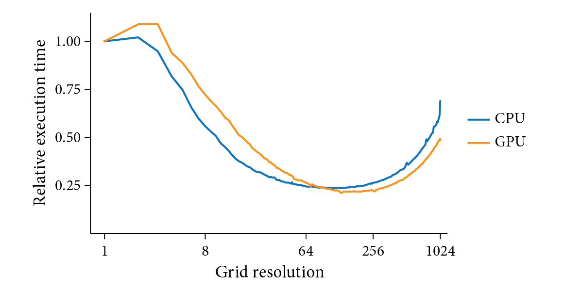
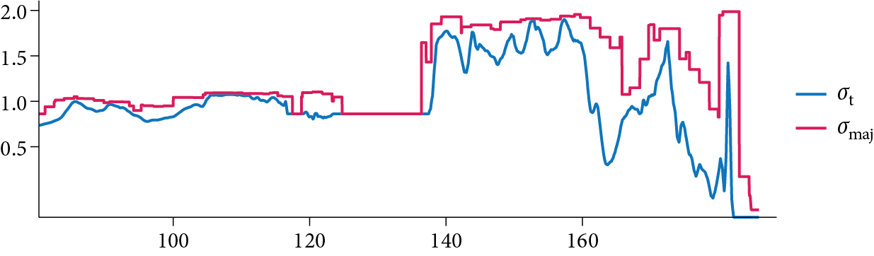
Although the grid can significantly improve the efficiency of volume sampling by providing majorants that are a better fit to the local medium density and thence reducing the number of null-scattering events, it also introduces the overhead of additional computations for stepping through voxels with the DDA. Too low a grid resolution and the majorants may not fit the volume well; too high a resolution and too much time will be spent walking through the grid. Figure 11.19 has a graph that illustrates these trade-offs, plotting voxel grid resolution versus execution time when rendering the cloud model used in Figures 11.2 and 11.8. We can see that the performance characteristics are similar on both the CPU and the GPU, with both exhibiting good performance with grid resolutions that span roughly 64 through 256 voxels on a side. Figure 11.20 shows the extinction coefficient and the majorant along a randomly selected ray that was traced when rendering the cloud scene; we can see that the majorants end up fitting the extinction coefficient well.

11.4.4 Uniform Grid Medium

The GridMedium stores medium densities and (optionally) emission at a regular 3D grid of positions, similar to the way that the image textures represent images with a 2D grid of samples.

The constructor takes a 3D array that stores the medium’s density and values that define emission as well as the medium space bounds of the grid and a transformation matrix that goes from medium space to rendering space. Most of its work is direct initialization of member variables, which we have elided here. Its one interesting bit is in the fragment <<Initialize majorantGrid for GridMedium>>, which we will see in a few pages.

Two steps give the and values for the medium at a point: first, baseline spectral values of these coefficients, sigma_a_spec and sigma_s_spec, are sampled at the specified wavelengths to give SampledSpectrum values for them. These are then scaled by the interpolated density from densityGrid. The phase function in this medium is uniform and parameterized only by the Henyey–Greenstein parameter.

The GridMedium allows volumetric emission to be specified in one of two ways. First, a grid of temperature values may be provided; these are interpreted as blackbody emission temperatures specified in degrees Kelvin (Section 4.4.1). Alternatively, a single general spectral distribution may be provided. Both are then scaled by values from the LeScale grid. Even though spatially varying general spectral distributions are not supported, these representations make it possible to specify a variety of emissive effects; Figure 11.5 uses blackbody emission and Figure 11.21 uses a scaled spectrum. An exercise at the end of the chapter outlines how this representation might be generalized.

A Boolean, isEmissive, indicates whether any emission has been specified. It is initialized in the GridMedium constructor, which makes the implementation of the IsEmissive() interface method easy.

The medium’s properties at a given point are found by interpolating values from the appropriate grids.

Initial values of and are found by sampling the baseline values.

Next, and are scaled by the interpolated density at p. The provided point must be transformed from rendering space to the medium’s space and then remapped to before the grid’s Lookup() method is called to interpolate the density.

If emission is present, the emitted radiance at the point is computed using whichever of the methods was used to specify it. The implementation here goes through some care to avoid calls to Lookup() when they are unnecessary, in order to improve performance.

Given a nonzero scale, whichever method is being used to specify emission is queried to get the SampledSpectrum.

As mentioned earlier, GridMedium uses DDAMajorantIterator to provide its majorants rather than using a single grid-wide majorant.

The GridMedium constructor concludes with the following fragment, which initializes a MajorantGrid with its majorants. Doing so is just a matter of iterating over all the majorant cells, computing their bounds, and finding the maximum density over them. The maximum density is easily found with a convenient SampledGrid method.

The implementation of the SampleRay() Medium interface method is now easy. We can find the overlap of the ray with the medium using a straightforward fragment, not included here, and compute the baseline value. With that, we have enough information to initialize the DDAMajorantIterator.

11.4.5 RGB Grid Medium

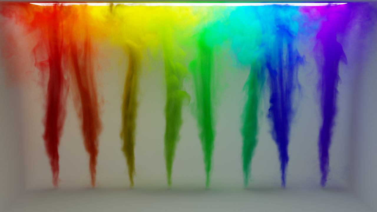
The last Medium implementation that we will describe is the RGBGridMedium. It is a variant of GridMedium that allows specifying the absorption and scattering coefficients as well as volumetric emission via RGB colors. This makes it possible to render a variety of colorful volumetric effects; an example is shown in Figure 11.22.

Its constructor, not included here, is similar to that of GridMedium in that most of what it does is to directly initialize member variables with values passed to it. As with GridMedium, the medium’s extent is jointly specified by a medium space bounding box and a transformation from medium space to rendering space.

Emission is specified by the combination of an optional SampledGrid of RGBIlluminantSpectrum values and a scale factor. The RGBGridMedium reports itself as emissive if the grid is present and the scale is nonzero. This misses the case of a fully zero LeGrid, though we assume that case to be unusual.

Sampling the medium at a point is mostly a matter of converting the various RGB values to SampledSpectrum values and trilinearly interpolating them to find their values at the lookup point p.

As with earlier Medium implementations, the phase function is uniform throughout this medium.

The absorption and scattering coefficients are stored using the RGBUnboundedSpectrum class. However, this class does not support the arithmetic operations that are necessary to perform trilinear interpolation in the SampledGrid::Lookup() method. For such cases, SampledGrid allows passing a callback function that converts the in-memory values to another type that does support them. Here, the implementation provides one that converts to SampledSpectrum, which does allow arithmetic and matches the type to be returned in MediumProperties as well.

Because sigmaScale is applied to both and , it provides a convenient way to fine-tune the density of a medium without needing to update all of its individual RGB values.

Volumetric emission is handled similarly, with a lambda function that converts the RGBIlluminantSpectrum values to SampledSpectrums for trilinear interpolation in the Lookup() method.

The DDAMajorantIterator provides majorants for the RGBGridMedium as well.

The MajorantGrid that is used by the DDAMajorantIterator is initialized by the following fragment, which runs at the end of the RGBGridMedium constructor.

Before explaining how the majorant grid voxels are initialized, we will discuss why RGBUnboundedSpectrum values are stored in rgbDensityGrid rather than the more obvious choice of RGB values. The most important reason is that the RGB to spectrum conversion approach from Section 4.6.6 does not guarantee that the spectral distribution’s value will always be less than or equal to the maximum of the original RGB components. Thus, storing RGB and setting majorants using bounds on RGB values would not give bounds on the eventual SampledSpectrum values that are computed.

One might nevertheless try to store RGB, convert those RGB values to spectra when initializing the majorant grid, and then bound those spectra to find majorants. That approach would also be unsuccessful, since when two RGB values are linearly interpolated, the corresponding RGBUnboundedSpectrum does not vary linearly between the RGBUnboundedSpectrum distributions of the two original RGB values.

Thus, RGBGridMedium stores RGBUnboundedSpectrum values at the grid sample points and linearly interpolates their SampledSpectrum values at lookup points. With that approach, we can guarantee that bounds on RGBUnboundedSpectrum values in a region of space (and then a bit more, given trilinear interpolation) give bounds on the sampled spectral values that are returned by SampledGrid::Lookup() in the SamplePoint() method, fulfilling the requirement for the majorant grid.

To compute the majorants, we use a SampledGrid method that returns its maximum value over a region of space and takes a lambda function that converts its underlying type to another—here, Float for the MajorantGrid.

One nit in how the majorants are computed is that the following code effectively assumes that the values in the and grids are independent. Although it computes a valid majorant, it is unable to account for cases like the two being defined such that for some constant . Then, the bound will be looser than it could be.

With the majorant grid initialized, the SampleRay() method’s implementation is trivial. (See Exercise 11.3 for a way in which it might be improved, however.)