14.3 Scattering from Layered Materials

In addition to describing scattering from larger-scale volumetric media like clouds or smoke, the equation of transfer can be used to model scattering at much smaller scales. The LayeredBxDF applies it to this task, implementing a reflection model that accounts for scattering from two interfaces that are represented by surfaces with independent BSDFs and with a medium between them. Monte Carlo can be applied to estimating the integrals that describe the aggregate scattering behavior, in a way similar to what is done in light transport algorithms. This approach is effectively the generalization of the technique used to sum up aggregate scattering from a pair of perfectly smooth dielectric interfaces in the ThinDielectricBxDF in Section 9.5.1.

Modeling surface reflectance as a composition of layers makes it possible to describe a variety of surfaces that are not well modeled by the BSDFs presented in Chapter 9. For example, automobile paint generally has a smooth reflective “clear coat” layer applied on top of it; the overall appearance of the paint is determined by the combination of light scattering from the layer’s interface as well as light scattering from the paint. (See Figure 14.11.) Tarnished metal can be modeled by an underlying metal BRDF with a thin scattering medium on top of it; it is again the aggregate result of a variety of light scattering paths that determines the overall appearance of the surface.

With general layered media, light may exit the surface at a different point than that at which it entered it. The LayeredBxDF does not model this effect but instead assumes that light enters and exits at the same point on the surface. (As a BxDF, it is unable to express any other sort of scattering, anyway.) This is a reasonable approximation if the distance between the two interfaces is relatively small. This approximation makes it possible to use a simplified 1D version of the equation of transfer. After deriving this variant, we will show its application to evaluating and sampling such BSDFs.

14.3.1 The One-Dimensional Equation of Transfer

Given plane-parallel 3D scattering media where the scattering properties are homogeneous across planes and only vary in depth, and where the incident illumination does not vary as a function of position over the medium’s planar boundary, the equations that describe scattering can be written in terms of 1D functions over depth (see Figure 14.12).

In this setting, the various quantities are more conveniently expressed as functions of depth rather than of distance along a ray. For example, if the extinction coefficient is given by , then the transmittance between two depths and for a ray with direction is

See Figure 14.13. This definition uses the fact that if a ray with direction travels a distance , then the change in is .

In the case of a homogeneous medium,

The 1D equation of transfer can be found in a similar fashion. It says that at points inside the medium the incident radiance at a depth in direction is given by

where is the depth of the medium interface that the ray from in direction intersects. (See Figure 14.14.) At boundaries, the incident radiance function is given by Equation (14.31) for directions that point into the medium. For directions that point outside it, incident radiance is found by integrating illumination from the scene.

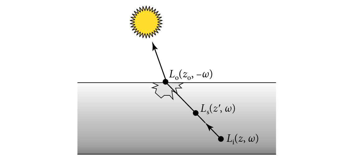
The scattering from an interface at a boundary of the medium is given by the incident radiance modulated by the boundary’s BSDF,

If we also assume there is no volumetric emission (as we will do in the LayeredBxDF), the source function in Equation (14.31) simplifies to

The LayeredBxDF further assumes that is constant over all wavelengths in the medium, which means that null scattering is not necessary for sampling distances in the medium. Null scattering is easily included in the 1D simplification of the equation of transfer if necessary, though we will not do so here. For similar reasons, we will also not derive its path integral form in 1D, though it too can be found with suitable simplifications to the approach that was used in Section 14.1.4. The “Further Reading” section has pointers to more details.

14.3.2 Layered BxDF

The equation of transfer describes the equilibrium distribution of radiance, though our interest here is in evaluating and sampling the BSDF that represents all the scattering from the layered medium. Fortunately, these two things can be connected. If we would like to evaluate the BSDF for a pair of directions and , then we can define an incident radiance function from a virtual light source from as

If a 1D medium is illuminated by such a light, then the outgoing radiance at the medium’s interface is equivalent to the value of the BSDF, (see Figure 14.15). One way to understand why this is so is to consider using such a light with the surface reflection equation:

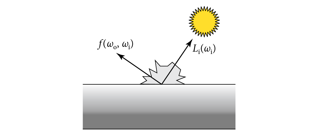
Thus, integrating the equation of transfer with such a light allows us to evaluate and sample the corresponding BSDF. However, this means that unlike all the BxDF implementations from Chapter 9, the values that LayeredBxDF returns from methods like f() and PDF() are stochastic. This is perfectly fine in the context of all of pbrt’s Monte Carlo–based techniques and does not affect the correctness of other estimators that use these values; it is purely one more source of error that can be controlled in a predictable way by increasing the number of samples.

The LayeredBxDF allows the specification of only two interfaces and a homogeneous participating medium between them. Figure 14.16 illustrates the geometric setting. Surfaces with more layers can be modeled using a LayeredBxDF where one or both of its layers are themselves LayeredBxDFs. (An exercise at the end of the chapter discusses a more efficient approach for supporting additional layers.)

The types of BxDFs at both interfaces can be provided as template parameters. While the user of a LayeredBxDF is free to provide a BxDF for both of these types (in which case pbrt’s regular dynamic dispatch mechanism will be used), performance is better if they are specific BxDFs and the compiler can generate a specialized implementation. This approach is used for the CoatedDiffuseBxDF and the CoatedConductorBxDF that are defined in Section 14.3.3. (The meaning of the twoSided template parameter will be explained in a few pages, where it is used.)

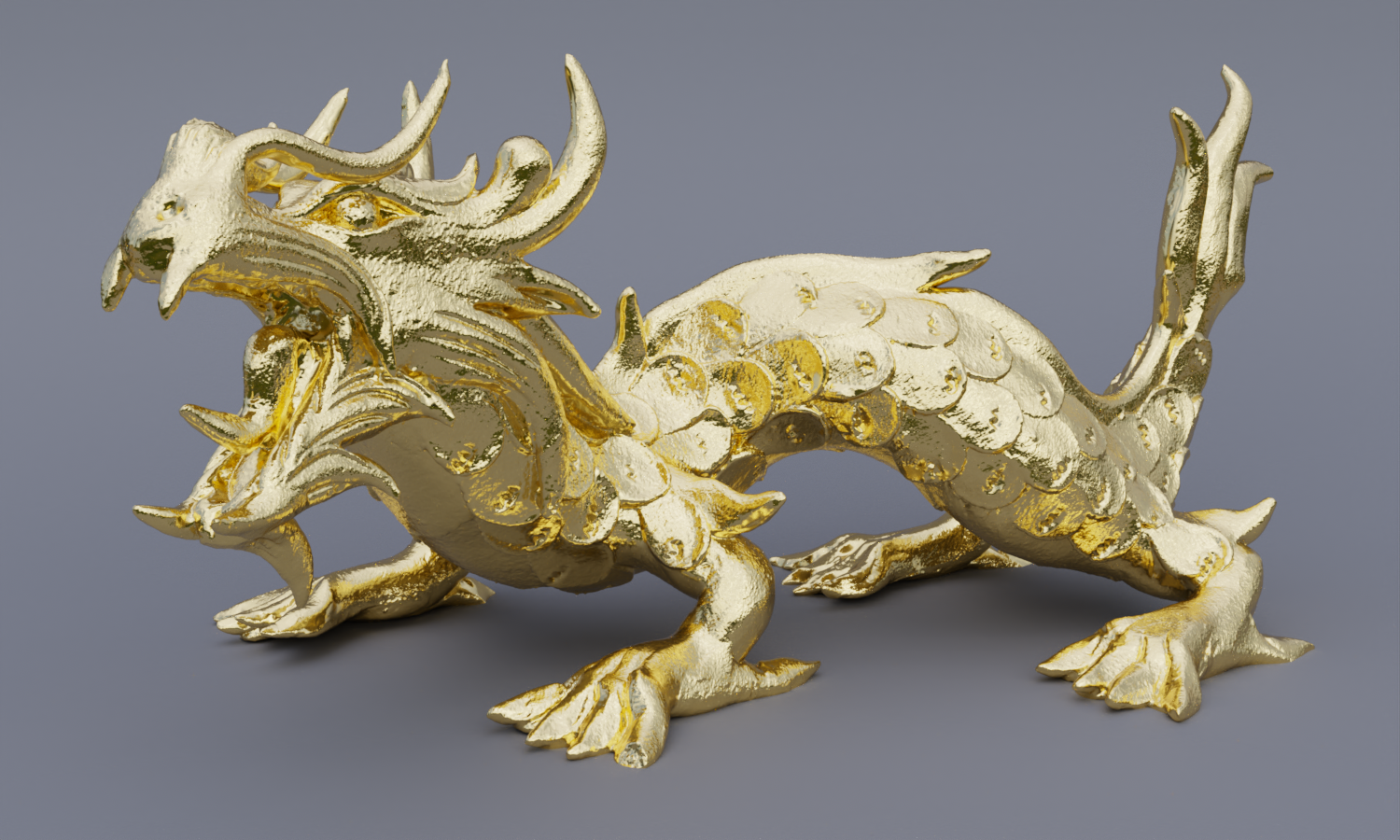
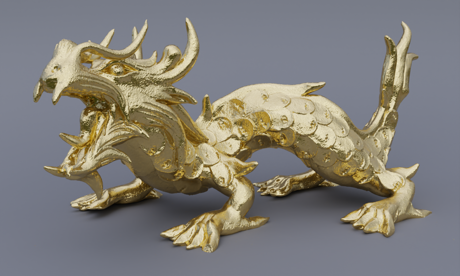
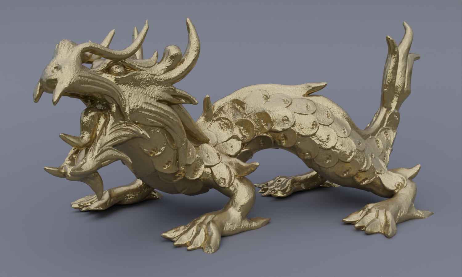
In addition to BxDFs for the two interfaces, the LayeredBxDF maintains member variables that describe the medium between them. Rather than have the user specify scattering coefficients, which can be unintuitive to set manually, it assumes a medium with and leaves it to the user to specify both the thickness of the medium and its scattering albedo. Figure 14.17 shows the effect of varying the thickness of the medium between a conductor base layer and a dielectric interface.

Two parameters control the Monte Carlo estimates. maxDepth has its usual role in setting a maximum number of scattering events along a path and nSamples controls the number of independent samples of the estimators that are averaged. Because additional samples in this context do not require tracing more rays or evaluating textures, it is more efficient to reduce any noise due to the stochastic BSDF by increasing this sampling rate rather than increasing the pixel sampling rate if a higher pixel sampling rate is not otherwise useful.

We will find it useful to have a helper function Tr() that returns the transmittance for a ray segment in the medium with given direction w that passes through a distance dz in , following Equation (14.30) with .

Although the LayeredBxDF is specified in terms of top and bottom interfaces, we will find it useful to exchange the “top” and “bottom” as necessary to have the convention that the interface that the incident ray intersects is defined to be the top one. (See Figure 14.18.) A helper class, TopOrBottomBxDF, manages the logic related to these possibilities. As its name suggests, it stores a pointer to one (and only one) of two BxDF types that are provided as template parameters.

TopOrBottomBxDF provides the implementation of a number of BxDF methods like f(), where it calls the corresponding method of whichever of the two BxDF types has been provided. In addition to f(), it has similar straightforward Sample_f(), PDF(), and Flags() methods, which we will not include here.

BSDF Evaluation

The BSDF evaluation method f() can now be implemented; it returns an average of the specified number of independent samples.

There is some preliminary computation that is independent of each sample taken to estimate the BSDF’s value. A few fragments take care of it before the random estimation begins.

With this BSDF, layered materials can be specified as either one- or two-sided via the twoSided template parameter. If a material is one-sided, then the shape’s surface normal is used to determine which interface an incident ray enters. If it is in the same hemisphere as the surface normal, it enters the top interface and otherwise it enters the bottom. This configuration is especially useful when both interfaces are transmissive and have different BSDFs.

For two-sided materials, the ray always enters the top interface. This option is useful when the bottom interface is opaque as is the case with the CoatedDiffuseBxDF, for example. In this case, it is usually desirable for scattering from both layers to be included, no matter which side the ray intersects.

One way to handle these options in the f() method would be to negate both directions and make a recursive call to f() if points below the surface and the material is two-sided. However, that solution is not a good one for the GPU, where it is likely to introduce thread divergence. (This topic is discussed in more detail in Section 15.1.1.) Therefore, both directions are negated at the start of the method and no recursive call is made in this case, which gives an equivalent result.

The next step is to determine which of the two BxDFs is the one that is encountered first by the incident ray. The sign of ’s component in the reflection coordinate system gives the answer.

It is also necessary to determine which interface exits. This is determined both by which interface enters and by whether and are in the same hemisphere. We end up with an unusual case where the exclusive-or operator comes in handy. Along the way, the method also stores which interface is the one that does not exit from. As random paths are sampled through the layers and medium, the implementation will always choose reflection from this interface and not transmission, as choosing the latter would end the path without being able to scatter out in the direction. The same logic then covers determining the depth at which the ray path will exit the surface.

If both directions are on the same side of the surface, then part of the BSDF’s value is given by reflection at the entrance interface. This can be evaluated directly by calling the interface’s BSDF’s f() method. The resulting value must be scaled by the total number of samples taken to estimate the BSDF in this method, since the final returned value is divided by nSamples.

pbrt’s BxDF interface does not include any uniform sample values as parameters to the f() method; there is no need for them for any of the other BxDFs in the system. In any case, an unbounded number of uniform random numbers are required for sampling operations when evaluating layered BSDFs. Therefore, f() initializes an RNG and defines a convenience lambda function that returns uniform random sample values. This does mean that the benefits of sampling with well-distributed point sets are not present here; an exercise at the end of the chapter returns to this issue.

The RNG is seeded carefully: it is important that calls to f() with different directions have different seeds so that there is no risk of errors due to correlation between the RNGs used for multiple samples in a pixel or across nearby pixels. However, we would also like the samples to be deterministic so that any call to f() with the same two directions always has the same set of random samples. This sort of reproducibility is important for debugging so that errors appear consistently across multiple runs of the program. Hashing the two provided directions along with the system-wide seed addresses all of these concerns.

In order to find the radiance leaving the interface in the direction , we need to integrate the product of the cosine-weighted BTDF at the interface with the incident radiance from inside the medium,

where is the hemisphere inside the medium (see Figure 14.19). The implementation uses the standard Monte Carlo estimator, taking a sample from the BTDF and then proceeding to estimate .

Sampling the direction is a case where it is useful to be able to specify to Sample_f() that only transmission should be sampled.

The task now is to compute a Monte Carlo estimate of the 1D equation of transfer, Equation (14.31). Before discussing how it is sampled, however, we will first consider some details related to the lighting calculation with the virtual light source. At each vertex of the path, we will want to compute the incident illumination due to the light. As shown in Figure 14.20, there are three factors in the light’s contribution: the value of the phase function or interface BSDF for a direction , the transmittance between the vertex and the exit interface, and the value of the interface’s BTDF for the direction from to .

Each of these three factors could be used for sampling; as before, one may sometimes be much more effective than the others. The LayeredBxDF implementation uses two of the three—sampling the phase function or BRDF at the current path vertex (as appropriate) and sampling the BTDF at the exit interface—and then weights the results using MIS.

There is no reason to repeatedly sample the exit interface BTDF at each path vertex since the direction is fixed. Therefore, the following fragment samples it once and holds on to the resulting BSDFSample. Note that the negation of the TransportMode parameter value mode is taken for the call to Sample_f(), which is important to reflect the fact that this sampling operation is following the reverse path with respect to sampling in terms of . This is an important detail so that the underlying BxDF can correctly account for non-symmetric scattering; see Section 9.5.2.

Moving forward to the random walk estimation of the equation of transfer, the implementation maintains the current path throughput weight beta, the depth z of the last scattering event, and the ray direction w.

We can now move to the body of the inner loop over scattering events along the path. After a Russian roulette test, a distance is sampled along the ray to determine the next path vertex either within the medium or at whichever interface the ray intersects.

It is worth considering terminating the path as the path throughput weight becomes low, though here the termination probability is set less aggressively than it was in the PathIntegrator and VolPathIntegrator. This reflects the fact that each bounce here is relatively inexpensive, so doing more work to improve the accuracy of the estimate is worthwhile.

The common case of no scattering in the medium is handled separately since it is much simpler than the case where volumetric scattering must be considered.

If there is no medium scattering, then only the first term of Equation (14.31) needs to be evaluated. The path vertices alternate between the two interfaces. Here beta is multiplied by the transmittance for the ray segment through the medium; the factor is found by estimating Equation (14.32), which will be handled shortly.

If the medium is scattering, we only sample one of the two terms of the 1D equation of transfer, choosing between taking a sample inside the medium and scattering at the other interface. A change in depth can be perfectly sampled from the 1D beam transmittance, Equation (14.30). Since , the PDF is

Given a depth found by adding or subtracting from the current depth according to the ray’s direction, medium scattering is chosen if is inside the medium and surface scattering is chosen otherwise. (The sampling scheme is thus similar to how the VolPathIntegrator chooses between medium and surface scattering.) In the case of scattering from an interface, the Clamp() call effectively forces to lie on whichever of the two interfaces the ray intersects next.

If is inside the medium, we have the estimator

Both the exponential factors and factors in and cancel, and we are left with simply the source function , which should be scaled by the path throughput. The following fragment adds an estimate of its value to the sum in f.

For a scattering event inside the medium, it is necessary to add the contribution of the virtual light source to the path radiance estimate and to sample a new direction to continue the path. For the MIS lighting sample based on sampling the interface’s BTDF, the outgoing direction from the path vertex is predetermined by the BTDF sample wis; all the factors of the path contribution are easily evaluated and the MIS weight is found using the PDF for the other sampling technique, sampling the phase function.

The second sampling strategy for the virtual light is based on sampling the phase function and then connecting to the virtual light source through the exit interface. Doing so shares some common work with sampling a new direction for the path, so the implementation takes the opportunity to update the path state after sampling the phase function here.

There is no reason to try connecting through the exit interface if the current ray direction is pointing away from it or if its BSDF is perfect specular.

If there is transmission through the interface, then because beta has already been updated to include the effect of scattering at , only the transmittance to the exit, MIS weight, and BTDF value need to be evaluated to compute the light’s contribution. One important detail in the following code is the ordering of arguments to the call to f() in the first line: due to the non-reciprocity of BTDFs, swapping these would lead to incorrect results. ^†

If no medium scattering event was sampled, the next path vertex is at an interface. In this case, the transmittance along the ray can be ignored: as before, the probability of evaluating the first term of Equation (14.31) has probability equal to and thus the two factors cancel, leaving us only needing to evaluate scattering at the boundary, Equation (14.32). The details differ depending on which interface the ray intersected.

If the ray intersected the exit interface, then it is only necessary to update the path throughput: no connection is made to the virtual light source since transmission through the exit interface to the light is accounted for by the lighting computation at the previous vertex. This fragment samples only the reflection component of the path here, since a ray that was transmitted outside the medium would end the path.

The <<Account for scattering at nonExitInterface>> fragment handles scattering from the other interface. It applies MIS to compute the contribution of the virtual light and samples a new direction with a form very similar to the case of scattering within the medium, just with the phase function replaced by the BRDF for evaluation and sampling. Therefore, we have not included its implementation here.

BSDF Sampling

The implementation of Sample_f() is generally similar to f(), so we will not include its implementation here, either. Its task is actually simpler: given the initial direction at one of the layer’s boundaries, it follows a random walk of scattering events through the layers and the medium, maintaining both the path throughput and the product of PDFs for each of the sampling decisions. When the random walk exits the medium, the outgoing direction is the sampled direction that is returned in the BSDFSample.

With this approach, it can be shown that the ratio of the path throughput to the PDF is equal to the ratio of the actual value of the BSDF and its PDF for the sampled direction (see the “Further Reading” section for details). Therefore, when the weighted path throughput is multiplied by the ratio of BSDFSample::f and BSDFSample::pdf, the correct weighting term is applied. (Review, for example, the fragment <<Update path state variables after surface scattering>> in the PathIntegrator.)

However, an implication of this is that the PDF value returned by Sample_f() cannot be used to compute the multiple importance sampling weight if the sampled ray hits an emissive surface; in that case, an independent estimate of the PDF must be computed via a call to the PDF() method. The BSDFSample::pdfIsProportional member variable flags this case and is set by Sample_f() here.

PDF Evaluation

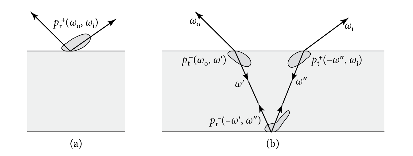
The PDF that corresponds to a LayeredBxDF’s BSDF can be expressed as an infinite sum. For example, consider the case of having a bottom layer that reflects light with BRDF and a top layer that both reflects light with BRDF and transmits it with BTDF , with an overall BSDF . If those BSDFs have associated PDFs and if scattering in the medium is neglected, then the overall PDF is

The first term gives the contribution for the PDF at the top interface and the second is the PDF for directions that were sampled via transmission through the top interface, scattering at the bottom, and then transmission back out in direction . Note the coupling of directions between the PDF factors in the integrand: the negation of the initial transmitted direction gives the first direction for evaluation of the base PDF , and so forth (see Figure 14.21). Subsequent terms of this sum account for light that is reflected back downward at the top interface instead of exiting the layers, and expressions of a similar form can be found for the PDF if the base layer is also transmissive.

It is possible to compute a stochastic estimate of the PDF by applying Monte Carlo to the integrals and by terminating the infinite sum using Russian roulette. For example, for the integral in Equation (14.36), we have the estimator

where is sampled from some distribution and from a distribution . There is great freedom in choosing the distributions and . However, as with algorithms like path tracing, care must be taken if some of the PDFs are Dirac delta distributions. For example, if the bottom layer is perfect specular, then will always be zero unless was sampled according to its PDF.

Consider what happens if is sampled using ’s sampling method, conditioned on , and if is sampled using ’s sampling method, conditioned on : the first and last probabilities in the numerator cancel with the probabilities in the denominator, and we are left simply with as the estimate; the effect of in the PDF is fully encapsulated by the distribution of directions used to evaluate .

A stochastic estimate of the PDF can be computed by following a random walk in a manner similar to the f() method, just with phase function and BSDF evaluation replaced with evaluations of the corresponding PDFs. However, because the PDF() method is only called to compute PDF values that are used for computing MIS weights, the implementation here will return an approximate PDF; doing so does not invalidate the MIS estimator. ^†

It is important that the RNG for the PDF() method is seeded differently than it is for the f() method, since it will often be called with the same pair of directions as are passed to f(), and we would like to be certain that there is no correlation between the results returned by the two of them.

If both directions are on the same side of the surface, then part of the full PDF is given by the PDF for reflection at the interface (this was the first term of Equation (14.36)). This component can be evaluated non-stochastically, assuming that the underlying PDF() methods are not themselves stochastic.

The more times light has been scattered, the more isotropic its directional distribution tends to become. We can take advantage of this fact by evaluating only the first term of the stochastic PDF estimate and modeling the remaining terms with a uniform distribution. We further neglect the effect of scattering in the medium, again under the assumption that if it is significant, a uniform distribution will be a suitable approximation.

If both directions are on the same side of the interface, then the remaining PDF integral is the double integral of the product of three PDFs that we considered earlier. We use the shorthand “TRT” for this case, corresponding to transmission, then reflection, then transmission.

We will apply two sampling strategies. The first is sampling both directions via tInterface, once conditioned on and once on —effectively a bidirectional approach. The second is sampling one direction via tInterface conditioned on and the other via rInterface conditioned on the first sampled direction. These are then combined using multiple importance sampling. After canceling factors and introducing an MIS weight , Equation (14.37) simplifies to

which is the estimator for both strategies.

Both sampling methods will use the wos sample while only one uses wis.

If tInterface is perfect specular, then there is no need to try sampling or to apply MIS. The PDF is all that remains from Equation (14.38).

Otherwise, we sample from as well. If that sample is from a perfect specular component, then again there is no need to use MIS and the estimator is just .

If neither interface has a specular sample, then both are combined. For the first sampling technique, the second factor cancels out as well and the estimator is times the MIS weight.

Similarly, for the second sampling technique, we are left with a PDF to evaluate and then weight using MIS.

The <<Evaluate TT term for PDF estimate>> fragment is of a similar form, so it is not included here.

The final returned PDF value has the PDF for uniform spherical sampling, , mixed with the estimate to account for higher-order terms.

14.3.3 Coated Diffuse and Coated Conductor Materials

Adding a dielectric interface on top of both diffuse materials and conductors is often useful to model surface reflection. For example, plastic can be modeled by putting such an interface above a diffuse material, and coated metals can be modeled by adding such an interface as well. In both cases, introducing a scattering layer can model effects like tarnish or weathering. Figure 14.22 shows the dragon model with a few variations of these.

pbrt provides both the CoatedDiffuseBxDF and the CoatedConductorBxDF for such uses. There is almost nothing to their implementations other than a public inheritance from LayeredBxDF with the appropriate types for the two interfaces.

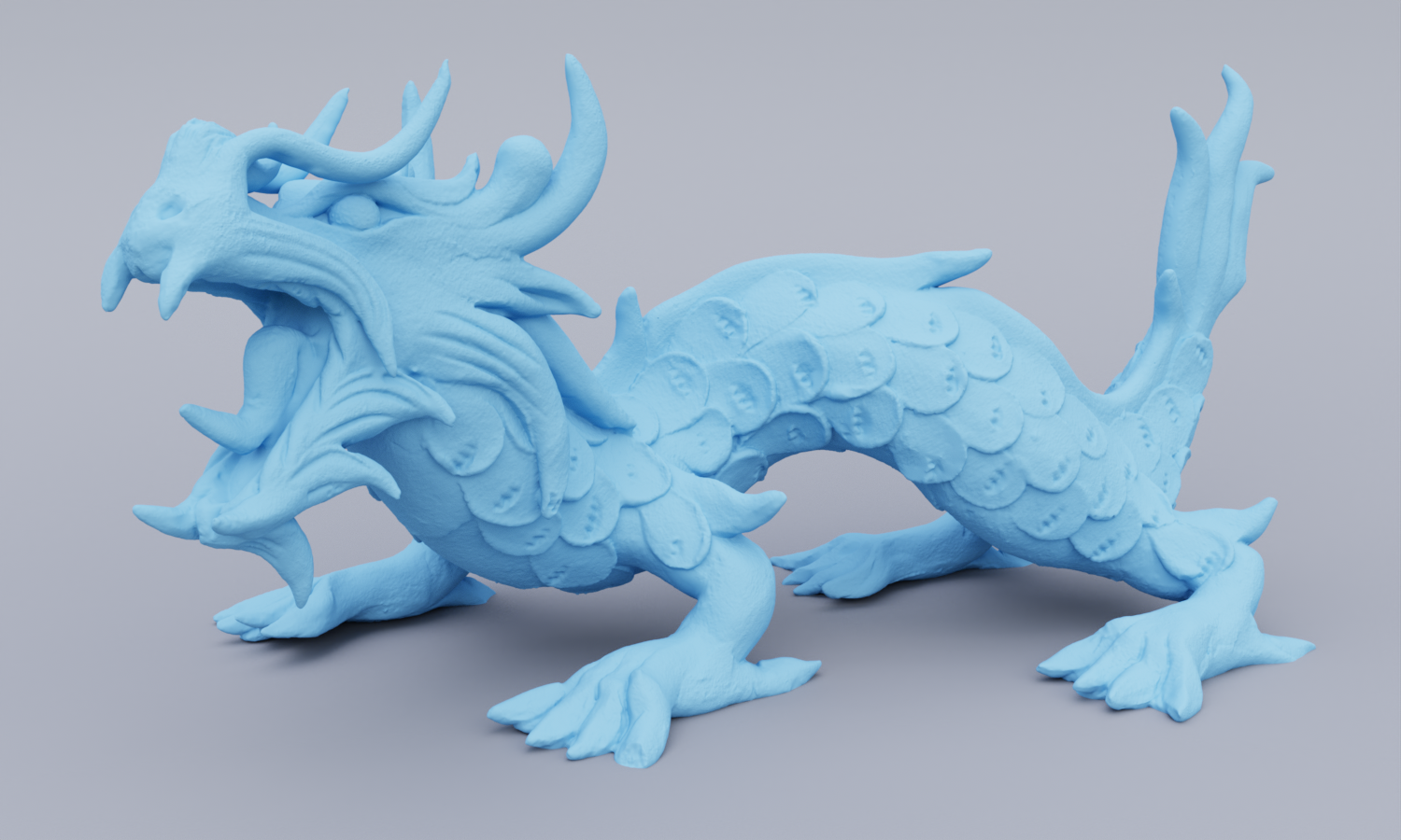
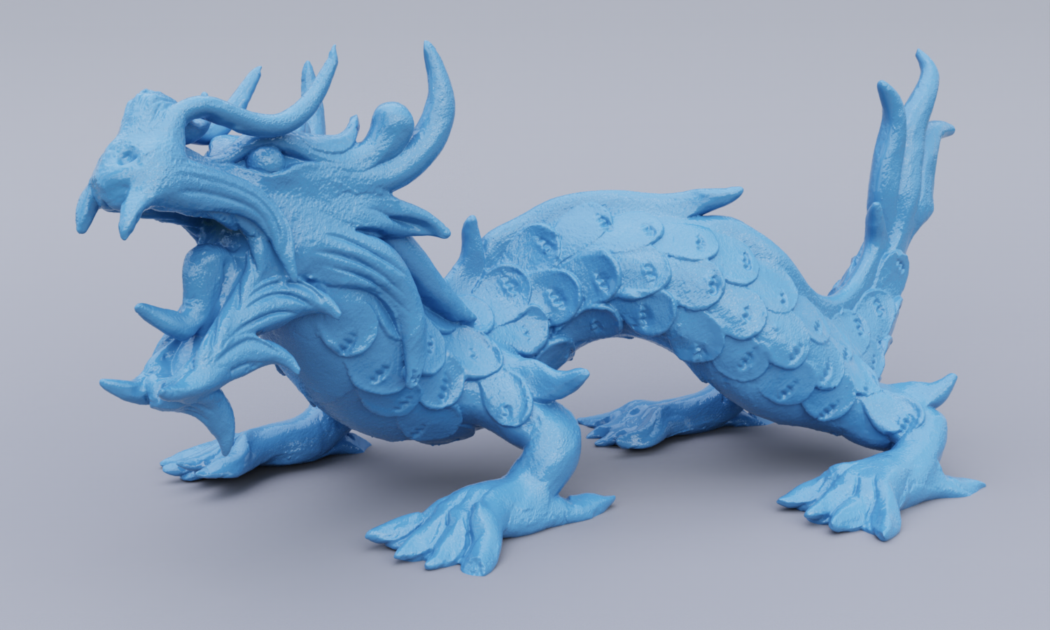
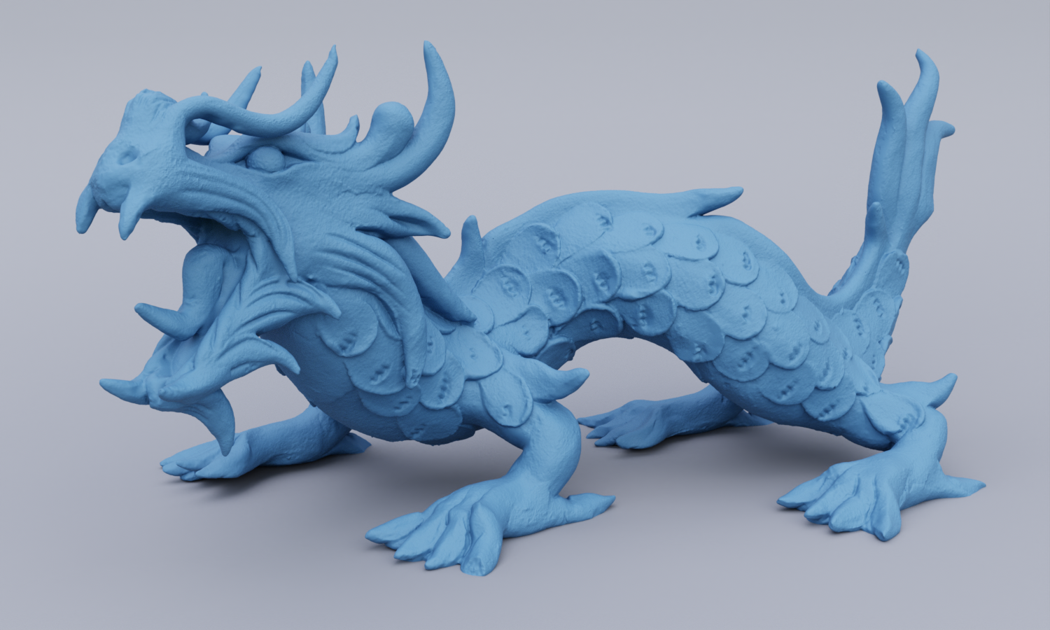
There are also corresponding Material implementations, CoatedDiffuseMaterial and CoatedConductorMaterial. Their implementations follow the familiar pattern of evaluating textures and then initializing the corresponding BxDF, and they are therefore not included here.