6.2 Spheres

Spheres are a special case of a general type of surface called quadrics—surfaces described by quadratic polynomials in , , and . They offer a good starting point for introducing ray intersection algorithms. In conjunction with a transformation matrix, pbrt’s Sphere shape can also take the form of an ellipsoid. pbrt supports two other basic types of quadrics: cylinders and disks. Other quadrics such as the cone, hyperboloid, and paraboloid are less useful for most rendering applications, and so are not included in the system.

Many surfaces can be described in one of two main ways: in implicit form and in parametric form. An implicit function describes a 3D surface as

The set of all points (, , ) that fulfill this condition defines the surface. For a unit sphere at the origin, the familiar implicit equation is . Only the set of points one unit from the origin satisfies this constraint, giving the unit sphere’s surface.

Many surfaces can also be described parametrically using a function to map 2D points to 3D points on the surface. For example, a sphere of radius can be described as a function of 2D spherical coordinates , where ranges from to and ranges from to (Figure 6.3):

We can transform this function into a function over and generalize it slightly to allow partial spheres that only sweep out and with the substitution

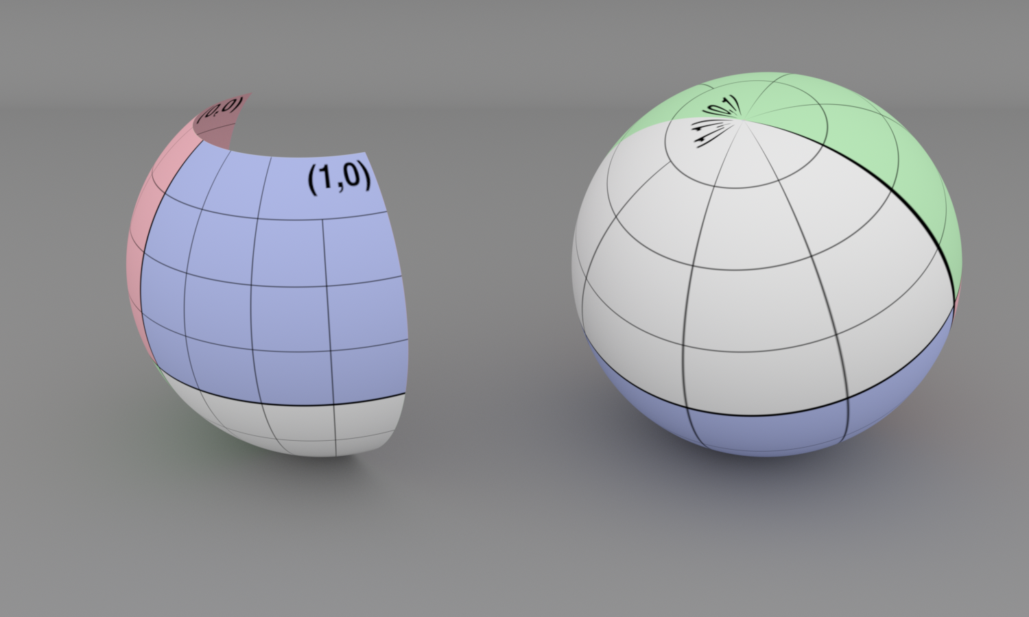
This form is particularly useful for texture mapping, where it can be directly used to map a texture defined over to the sphere. Figure 6.4 shows an image of two spheres; a grid image map has been used to show the parameterization.

As we describe the implementation of the sphere shape, we will make use of both the implicit and parametric descriptions of the shape, depending on which is a more natural way to approach the particular problem we are facing.

The Sphere class represents a sphere that is centered at the origin. As with all the other shapes, its implementation is in the files shapes.h and shapes.cpp.

As mentioned earlier, spheres in pbrt are defined in a coordinate system where the center of the sphere is at the origin. The sphere constructor is provided transformations that map between the sphere’s object space and rendering space.

Although pbrt supports animated transformation matrices, the transformations here are not AnimatedTransforms. (Such is also the case for all the shapes defined in this chapter.) Animated shape transformations are instead handled by using a TransformedPrimitive to represent the shape in the scene. Doing so allows us to centralize some of the tricky details related to animated transformations in a single place, rather than requiring all Shapes to handle this case.

The radius of the sphere can have an arbitrary positive value, and the sphere’s extent can be truncated in two different ways. First, minimum and maximum values may be set; the parts of the sphere below and above these planes, respectively, are cut off. Second, considering the parameterization of the sphere in spherical coordinates, a maximum value can be set. The sphere sweeps out values from 0 to the given such that the section of the sphere with spherical values above is also removed.

Finally, the Sphere constructor also takes a Boolean parameter, reverseOrientation, that indicates whether their surface normal directions should be reversed from the default (which is pointing outside the sphere). This capability is useful because the orientation of the surface normal is used to determine which side of a shape is “outside.” For example, shapes that emit illumination are by default emissive only on the side the surface normal lies on. The value of this parameter is managed via the ReverseOrientation statement in pbrt scene description files.

6.2.1 Bounding

Computing an object-space bounding box for a sphere is straightforward. The implementation here uses the values of and provided by the user to tighten up the bound when less than an entire sphere is being rendered. However, it does not do the extra work to compute a tighter bounding box when is less than . This improvement is left as an exercise. This object-space bounding box is transformed to rendering space before being returned.

The Sphere’s NormalBounds() method does not consider any form of partial spheres but always returns the bounds for an entire sphere, which is all possible directions.

6.2.2 Intersection Tests

The ray intersection test is broken into two stages. First, BasicIntersect() does the basic ray–sphere intersection test and returns a small structure, QuadricIntersection, if an intersection is found. A subsequent call to the InteractionFromIntersection() method transforms the QuadricIntersection into a full-blown SurfaceInteraction, which can be returned from the Intersection() method.

There are two motivations for separating the intersection test into two stages like this. One is that doing so allows the IntersectP() method to be implemented as a trivial wrapper around BasicIntersect(). The second is that pbrt’s GPU rendering path is organized such that the closest intersection among all shapes is found before the full SurfaceInteraction is constructed; this decomposition fits that directly.

QuadricIntersection stores the parametric along the ray where the intersection occurred, the object-space intersection point, and the sphere’s value there. As its name suggests, this structure will be used by the other quadrics in the same way it is here.

The basic intersection test transforms the provided rendering-space ray to object space and intersects it with the complete sphere. If a partial sphere has been specified, some additional tests reject intersections with portions of the sphere that have been removed.

The transformed ray origin and direction are respectively stored using Point3fi and Vector3fi classes rather than the usual Point3f and Vector3f. These classes represent those quantities as small intervals in each dimension that bound the floating-point round-off error that was introduced by applying the transformation. Later, we will see that these error bounds will be useful for improving the geometric accuracy of the intersection computation. For the most part, these classes can respectively be used just like Point3f and Vector3f.

If a sphere is centered at the origin with radius , its implicit representation is

By substituting the parametric representation of the ray from Equation (3.4) into the implicit sphere equation, we have

Note that all elements of this equation besides are known values. The values where the equation holds give the parametric positions along the ray where the implicit sphere equation is satisfied and thus the points along the ray where it intersects the sphere. We can expand this equation and gather the coefficients for a general quadratic equation in ,

where ^†

The Interval class stores a small range of floating-point values to maintain bounds on floating-point rounding error. It is defined in Section B.2.15 and is analogous to Float in the way that Point3fi is to Point3f, for example.

Given Interval, Equation (6.3) directly translates to the following fragment of source code.

The fragment <<Compute sphere quadratic discriminant discrim>> computes the discriminant in a way that maintains numerical accuracy in tricky cases. It is defined later, in Section 6.8.3, after related topics about floating-point arithmetic have been introduced. Proceeding here with its value in discrim, the quadratic equation can be applied. Here we use a variant of the traditional approach that gives more accuracy; it is described in Section B.2.10.

Because t0 and t1 represent intervals of floating-point values, it may be ambiguous which of them is less than the other. We use their lower bound for this test, so that in ambiguous cases, at least we do not risk returning a hit that is potentially farther away than an actual closer hit.

A similar ambiguity must be accounted for when testing the values against the acceptable range. In ambiguous cases, we err on the side of returning no intersection rather than an invalid one. The closest valid is then stored in tShapeHit.

Given the parametric distance along the ray to the intersection with a full sphere, the intersection point pHit can be computed as that offset along the ray. In its initializer, all the respective interval types are cast back to their non-interval equivalents, which gives their midpoint. (The remainder of the intersection test no longer needs the information provided by the intervals.) Due to floating-point precision limitations, this computed intersection point pHit may lie a bit to one side of the actual sphere surface; the <<Refine sphere intersection point>> fragment, which is defined in Section 6.8.5, improves the accuracy of this value.

It is next necessary to handle partial spheres with clipped or ranges—intersections that are in clipped areas must be ignored. The implementation starts by computing the value for the hit point. Using the parametric representation of the sphere,

so . It is necessary to remap the result of the standard library’s std::atan() function to a value between and , to match the sphere’s original definition.

The hit point can now be tested against the specified minima and maxima for and . One subtlety is that it is important to skip the tests if the range includes the entire sphere; the computed pHit.z value may be slightly out of the range due to floating-point round-off, so we should only perform this test when the user expects the sphere to be partially incomplete. If the intersection is not valid, the routine tries again with .

At this point in the routine, it is certain that the ray hits the sphere. A QuadricIntersection is returned that encapsulates sufficient information about it to determine the rest of the geometric information at the intersection point. Recall from Section 6.1.4 that even though tShapeHit was computed in object space, it is also the correct value in rendering space. Therefore, it can be returned directly.

With BasicIntersect() implemented, Sphere::IntersectP() is easily taken care of.

A QuadricIntersection can be upgraded to a SurfaceInteraction with a call to InteractionFromIntersection().

The method first computes and values by scaling the previously computed value for the hit to lie between 0 and 1 and by computing a value between 0 and 1 for the hit point based on the range of values for the given sphere. Then it finds the parametric partial derivatives of position and and surface normal and .

Computing the partial derivatives of a point on the sphere is a short exercise in algebra. Here we will show how the component of , , is calculated; the other components are found similarly. Using the parametric definition of the sphere, we have

Using a substitution based on the parametric definition of the sphere’s coordinate, this simplifies to

Similarly,

and

A similar process gives . The complete result is

and the implementation follows directly.

It is also useful to determine how the normal changes as we move along the surface in the and directions. (For example, the antialiasing techniques in Chapter 10 use this information to antialias textures on objects that are seen reflected in curved surfaces.) The differential changes in normal and are given by the Weingarten equations from differential geometry:

where , , and are coefficients of the first fundamental form and are given by

These are easily computed with the and values found earlier. The , , and are coefficients of the second fundamental form,

The two fundamental forms capture elementary metric properties of a surface, including notions of distance, angle, and curvature; see a differential geometry textbook such as Gray (1993) for details. To find , , and , it is necessary to compute the second-order partial derivatives and so on.

For spheres, a little more algebra gives the second derivatives:

The translation into code is straightforward.

Given all the partial derivatives, it is also easy to compute the coefficients of the fundamental forms.

We now have all the values necessary to apply the Weingarten equations. For this computation, we have found it worthwhile to use DifferenceOfProducts() to compute for the greater numerical accuracy it provides than the direct expression of that computation. Note also that we must be careful to avoid dividing by 0 if that expression is zero-valued so that dndu and dndv do not take on not-a-number values in that case.

Having computed the surface parameterization and all the relevant partial derivatives, a SurfaceInteraction structure that contains all the necessary geometric information for this intersection can be returned. There are three things to note in the parameter values passed to the SurfaceInteraction constructor.

1. The intersection point is provided as a Point3i that takes the pHit point computed earlier and an error bound pError that is initialized in the fragment <<Compute error bounds for sphere intersection>>, which is defined later, in Section 6.8.5.
2. The SurfaceInteraction is initialized with object-space geometric quantities (pHit, dpdu, etc.) and is then transformed to rendering space when it is returned. However, one of the parameters is the outgoing direction, . This is passed in to InteractionFromIntersection(), but must be transformed to object space before being passed to the constructor so that the returned Interaction::wo value is in rendering space again.
3. The flipNormal parameter indicates whether the surface normal should be flipped after it is initially computed with the cross product of dpdu and dpdv. This should be done either if the ReverseOrientation directive has been enabled or if the object-to-rendering-space transform swaps coordinate system handedness (but not if both of these are the case). (The need for the latter condition was discussed in Section 3.11.1.)

6.2.3 Surface Area

To compute the surface area of quadrics, we use a standard formula from integral calculus. If a curve from to is revolved around the axis, the surface area of the resulting swept surface is

where denotes the derivative . Since most of our surfaces of revolution are only partially swept around the axis, we will instead use the formula

The sphere is a surface of revolution of a circular arc. The function that defines the profile curve along the axis of the sphere is

and its derivative is

Recall that the sphere is clipped at and . The surface area is therefore

For the full sphere , , and , so we have the standard formula , confirming that the formula makes sense.

6.2.4 Sampling

Uniformly sampling a point on the sphere’s area is easy: Sphere::Sample() generates a point on the unit sphere using SampleUniformSphere() and then scales the point by the sphere’s radius. A bound on the numeric error in this value is found in a fragment that will be defined later.

Because the object-space sphere is at the origin, the object-space surface normal is easily found by converting the object-space point to a normal vector and then normalizing it. A Point3fi for the sample point can be initialized from pObj and its error bounds. The final sample is returned in rendering space with a PDF equal to one over the surface area, since this Sample() method samples uniformly by surface area.

The parametric coordinates for the point are given by inverting Equations (6.1) and (6.2).

The associated PDF() method returns the same PDF.

For the sphere sampling method that is given a point being illuminated, we can do much better than sampling over the sphere’s entire area. While uniform sampling over its surface would be perfectly correct, a better approach is not to sample points on the sphere that are definitely not visible (such as those on the back side of the sphere as seen from the point). The sampling routine here instead uniformly samples directions over the solid angle subtended by the sphere from the reference point and then computes the point on the sphere corresponding to the sampled direction.

For points that lie inside the sphere, the entire sphere should be sampled, since the whole sphere is visible from inside it. Note that the reference point used in this determination, pOrigin, is computed using the OffsetRayOrigin() function. Doing so ensures that if the reference point came from a ray intersecting the sphere, the point tested does not lie on the wrong side of the sphere due to rounding error.

A call to the first Sample() method gives an initial ShapeSample for a point on the sphere. The direction vector from the reference point to the sampled point wi is computed and then normalized, so long as it is non-degenerate.

To compute the value of the PDF, the method converts the value of the PDF with respect to surface area from the call to Sample() to a PDF with respect to solid angle from the reference point. Doing so requires division by the factor

where is the angle between the direction of the ray from the point on the light to the reference point and the light’s surface normal, and is the distance between the point on the light and the point being shaded (recall the discussion about transforming between area and directional integration domains in Section 4.2.3).

In the rare case that the surface normal and wi are perpendicular, this results in an infinite value, in which case no valid sample is returned.

For the more common case of a point outside the sphere, sampling within the cone proceeds.

If the reference point is outside the sphere, then as seen from the reference point the sphere subtends an angle

where is the radius of the sphere and is its center (Figure 6.5). The sampling method here computes the cosine of the subtended angle using Equation (6.4) and then uniformly samples directions inside this cone of directions using an approach that is derived for the SampleUniformCone() function in Section A.5.4, sampling an offset from the center vector and then uniformly sampling a rotation angle around the vector. That function is not used here, however, as we will need some of the intermediate values in the following fragments.

As shown in Section A.5.4, uniform sampling of between and 1 gives the cosine of a uniformly sampled direction in the cone.

For very small angles, is close to one. Computing by subtracting this value from 1 gives a value close to 0, but with very little accuracy, since there is much less floating-point precision close to 1 than there is by 0. Therefore, in this case, we use single-term Taylor expansions near 0 to compute and related terms, which gives much better accuracy.

Given a sample angle with respect to the sampling coordinate system computed earlier, we can directly compute the corresponding point on the sphere. The first step is to find the angle between the vector from the reference point to the sampled point on the sphere and the vector from the center of the sphere to . The basic setting is shown in Figure 6.6.

We denote the distance from the reference point to the center of the sphere by . Applying the law of sines, we can find that

Because is an obtuse angle, . Given two of the three angles of the triangle, it follows that

We can avoid expensive inverse trigonometric functions by taking advantage of the fact that we only need the sine and cosine of . If we take the cosine of both sides of this equation, apply the cosine angle addition formula, and then use the two relationships and , we can find

The value of follows from the identity .

The angle and give the spherical coordinates for the sampled direction with respect to a coordinate system with axis centered around the vector from the reference point to the sphere center. We can use an instance of the Frame class to transform the direction from that coordinate system to rendering space. The surface normal on the sphere can then be computed as the negation of that vector and the point on the sphere can be found by scaling by the radius and translating by the sphere’s center point.

The <<Compute coordinates for sampled point on sphere>> fragment applies the same mapping using the object space sampled point as is done in the Intersect() method, and so it is elided. The PDF for uniform sampling in a cone is . (A derivation is in Section A.5.4.)

The method that computes the PDF for sampling a direction toward a sphere from a reference point also differs depending on which of the two sampling strategies would be used for the point.

If the reference point is inside the sphere, a uniform area sampling strategy would have been used.

First, the corresponding point on the sphere is found by intersecting a ray leaving the reference point in direction wi with the sphere. Note that this is a fairly efficient computation since it is only intersecting the ray with a single sphere and not the entire scene.

In turn, the uniform area density of one over the surface area is converted to a solid angle density following the same approach as was used in the previous Sample() method.

The value of the PDF is easily computed using the same trigonometric identities as were used in the sampling routine.

Here it is also worth considering numerical accuracy when the sphere subtends a small solid angle from the reference point. In that case, cosThetaMax will be close to 1 and the value of oneMinusCosThetaMax will be relatively inaccurate; we then switch to the one-term Taylor approximation of , which is more accurate near zero.