1.2 Photorealistic Rendering and the Ray-Tracing Algorithm

The goal of photorealistic rendering is to create an image of a 3D scene that is indistinguishable from a photograph of the same scene. Before we describe the rendering process, it is important to understand that in this context the word indistinguishable is imprecise because it involves a human observer, and different observers may perceive the same image differently. Although we will cover a few perceptual issues in this book, accounting for the precise characteristics of a given observer is a difficult and not fully solved problem. For the most part, we will be satisfied with an accurate simulation of the physics of light and its interaction with matter, relying on our understanding of display technology to present the best possible image to the viewer.

Given this single-minded focus on realistic simulation of light, it seems prudent to ask: what is light? Perception through light is central to our very existence, and this simple question has thus occupied the minds of famous philosophers and physicists since the beginning of recorded time. The ancient Indian philosophical school of Vaisheshika (5th–6th century BC) viewed light as a collection of small particles traveling along rays at high velocity. In the fifth century BC, the Greek philosopher Empedocles postulated that a divine fire emerged from human eyes and combined with light rays from the sun to produce vision. Between the 18th and 19th century, polymaths such as Isaac Newton, Thomas Young, and Augustin-Jean Fresnel endorsed conflicting theories modeling light as the consequence of either wave or particle propagation. During the same time period, André-Marie Ampère, Joseph-Louis Lagrange, Carl Friedrich Gauß, and Michael Faraday investigated the relations between electricity and magnetism that culminated in a sudden and dramatic unification by James Clerk Maxwell into a combined theory that is now known as electromagnetism.

Light is a wave-like manifestation in this framework: the motion of electrically charged particles such as electrons in a light bulb’s filament produces a disturbance of a surrounding electric field that propagates away from the source. The electric oscillation also causes a secondary oscillation of the magnetic field, which in turn reinforces an oscillation of the electric field, and so on. The interplay of these two fields leads to a self-propagating wave that can travel extremely large distances: millions of light years, in the case of distant stars visible in a clear night sky. In the early 20th century, work by Max Planck, Max Born, Erwin Schrödinger, and Werner Heisenberg led to another substantial shift of our understanding: at a microscopic level, elementary properties like energy and momentum are quantized, which means that they can only exist as an integer multiple of a base amount that is known as a quantum. In the case of electromagnetic oscillations, this quantum is referred to as a photon. In this sense, our physical understanding has come full circle: once we turn to very small scales, light again betrays a particle-like behavior that coexists with its overall wave-like nature.

How does our goal of simulating light to produce realistic images fit into all of this? Faced with this tower of increasingly advanced explanations, a fundamental question arises: how far must we climb this tower to attain photorealism? To our great fortune, the answer turns out to be “not far at all.” Waves comprising visible light are extremely small, measuring only a few hundred nanometers from crest to trough. The complex wave-like behavior of light appears at these small scales, but it is of little consequence when simulating objects at the scale of, say, centimeters or meters. This is excellent news, because detailed wave-level simulations of anything larger than a few micrometers are impractical: computer graphics would not exist in its current form if this level of detail was necessary to render images. Instead, we will mostly work with equations developed between the 16th and early 19th century that model light as particles that travel along rays. This leads to a more efficient computational approach based on a key operation known as ray tracing.

Ray tracing is conceptually a simple algorithm; it is based on following the path of a ray of light through a scene as it interacts with and bounces off objects in an environment. Although there are many ways to write a ray tracer, all such systems simulate at least the following objects and phenomena:

• Cameras: A camera model determines how and from where the scene is being viewed, including how an image of the scene is recorded on a sensor. Many rendering systems generate viewing rays starting at the camera that are then traced into the scene to determine which objects are visible at each pixel.
• Ray–object intersections: We must be able to tell precisely where a given ray intersects a given geometric object. In addition, we need to determine certain properties of the object at the intersection point, such as a surface normal or its material. Most ray tracers also have some facility for testing the intersection of a ray with multiple objects, typically returning the closest intersection along the ray.
• Light sources: Without lighting, there would be little point in rendering a scene. A ray tracer must model the distribution of light throughout the scene, including not only the locations of the lights themselves but also the way in which they distribute their energy throughout space.
• Visibility: In order to know whether a given light deposits energy at a point on a surface, we must know whether there is an uninterrupted path from the point to the light source. Fortunately, this question is easy to answer in a ray tracer, since we can just construct the ray from the surface to the light, find the closest ray–object intersection, and compare the intersection distance to the light distance.
• Light scattering at surfaces: Each object must provide a description of its appearance, including information about how light interacts with the object’s surface, as well as the nature of the reradiated (or scattered) light. Models for surface scattering are typically parameterized so that they can simulate a variety of appearances.
• Indirect light transport: Because light can arrive at a surface after bouncing off or passing through other surfaces, it is usually necessary to trace additional rays to capture this effect.
• Ray propagation: We need to know what happens to the light traveling along a ray as it passes through space. If we are rendering a scene in a vacuum, light energy remains constant along a ray. Although true vacuums are unusual on Earth, they are a reasonable approximation for many environments. More sophisticated models are available for tracing rays through fog, smoke, the Earth’s atmosphere, and so on.

We will briefly discuss each of these simulation tasks in this section. In the next section, we will show pbrt’s high-level interface to the underlying simulation components and will present a simple rendering algorithm that randomly samples light paths through a scene in order to generate images.

1.2.1 Cameras and Film

Nearly everyone has used a camera and is familiar with its basic functionality: you indicate your desire to record an image of the world (usually by pressing a button or tapping a screen), and the image is recorded onto a piece of film or by an electronic sensor. ^† One of the simplest devices for taking photographs is called the pinhole camera. Pinhole cameras consist of a light-tight box with a tiny hole at one end (Figure 1.2). When the hole is uncovered, light enters and falls on a piece of photographic paper that is affixed to the other end of the box. Despite its simplicity, this kind of camera is still used today, mostly for artistic purposes. Long exposure times are necessary to get enough light on the film to form an image.

Although most cameras are substantially more complex than the pinhole camera, it is a convenient starting point for simulation. The most important function of the camera is to define the portion of the scene that will be recorded onto the film. In Figure 1.2, we can see how connecting the pinhole to the edges of the film creates a double pyramid that extends into the scene. Objects that are not inside this pyramid cannot be imaged onto the film. Because actual cameras image a more complex shape than a pyramid, we will refer to the region of space that can potentially be imaged onto the film as the viewing volume.

Another way to think about the pinhole camera is to place the film plane in front of the pinhole but at the same distance (Figure 1.3). Note that connecting the hole to the film defines exactly the same viewing volume as before. Of course, this is not a practical way to build a real camera, but for simulation purposes it is a convenient abstraction. When the film (or image) plane is in front of the pinhole, the pinhole is frequently referred to as the eye.

Now we come to the crucial issue in rendering: at each point in the image, what color does the camera record? The answer to this question is partially determined by what part of the scene is visible at that point. If we recall the original pinhole camera, it is clear that only light rays that travel along the vector between the pinhole and a point on the film can contribute to that film location. In our simulated camera with the film plane in front of the eye, we are interested in the amount of light traveling from the image point to the eye.

Therefore, an important task of the camera simulator is to take a point on the image and generate rays along which incident light will contribute to that image location. Because a ray consists of an origin point and a direction vector, this task is particularly simple for the pinhole camera model of Figure 1.3: it uses the pinhole for the origin and the vector from the pinhole to the imaging plane as the ray’s direction. For more complex camera models involving multiple lenses, the calculation of the ray that corresponds to a given point on the image may be more involved.

Light arriving at the camera along a ray will generally carry different amounts of energy at different wavelengths. The human visual system interprets this wavelength variation as color. Most camera sensors record separate measurements for three wavelength distributions that correspond to red, green, and blue colors, which is sufficient to reconstruct a scene’s visual appearance to a human observer. (Section 4.6 discusses color in more detail.) Therefore, cameras in pbrt also include a film abstraction that both stores the image and models the film sensor’s response to incident light.

pbrt’s camera and film abstraction is described in detail in Chapter 5. With the process of converting image locations to rays encapsulated in the camera module and with the film abstraction responsible for determining the sensor’s response to light, the rest of the rendering system can focus on evaluating the lighting along those rays.

1.2.2 Ray–Object Intersections

Each time the camera generates a ray, the first task of the renderer is to determine which object, if any, that ray intersects first and where the intersection occurs. This intersection point is the visible point along the ray, and we will want to simulate the interaction of light with the object at this point. To find the intersection, we must test the ray for intersection against all objects in the scene and select the one that the ray intersects first. Given a ray , we first start by writing it in parametric form:

where is the ray’s origin, is its direction vector, and is a parameter whose legal range is . We can obtain a point along the ray by specifying its parametric value and evaluating the above equation.

It is often easy to find the intersection between the ray and a surface defined by an implicit function . We first substitute the ray equation into the implicit equation, producing a new function whose only parameter is . We then solve this function for and substitute the smallest positive root into the ray equation to find the desired point. For example, the implicit equation of a sphere centered at the origin with radius  is

Substituting the ray equation, we have

where subscripts denote the corresponding component of a point or vector. For a given ray and a given sphere, all the values besides are known, giving us an easily solved quadratic equation in . If there are no real roots, the ray misses the sphere; if there are roots, the smallest positive one gives the intersection point.

The intersection point alone is not enough information for the rest of the ray tracer; it needs to know certain properties of the surface at the point. First, a representation of the material at the point must be determined and passed along to later stages of the ray-tracing algorithm. Second, additional geometric information about the intersection point will also be required in order to shade the point. For example, the surface normal is always required. Although many ray tracers operate with only , more sophisticated rendering systems like pbrt require even more information, such as various partial derivatives of position and surface normal with respect to the local parameterization of the surface.

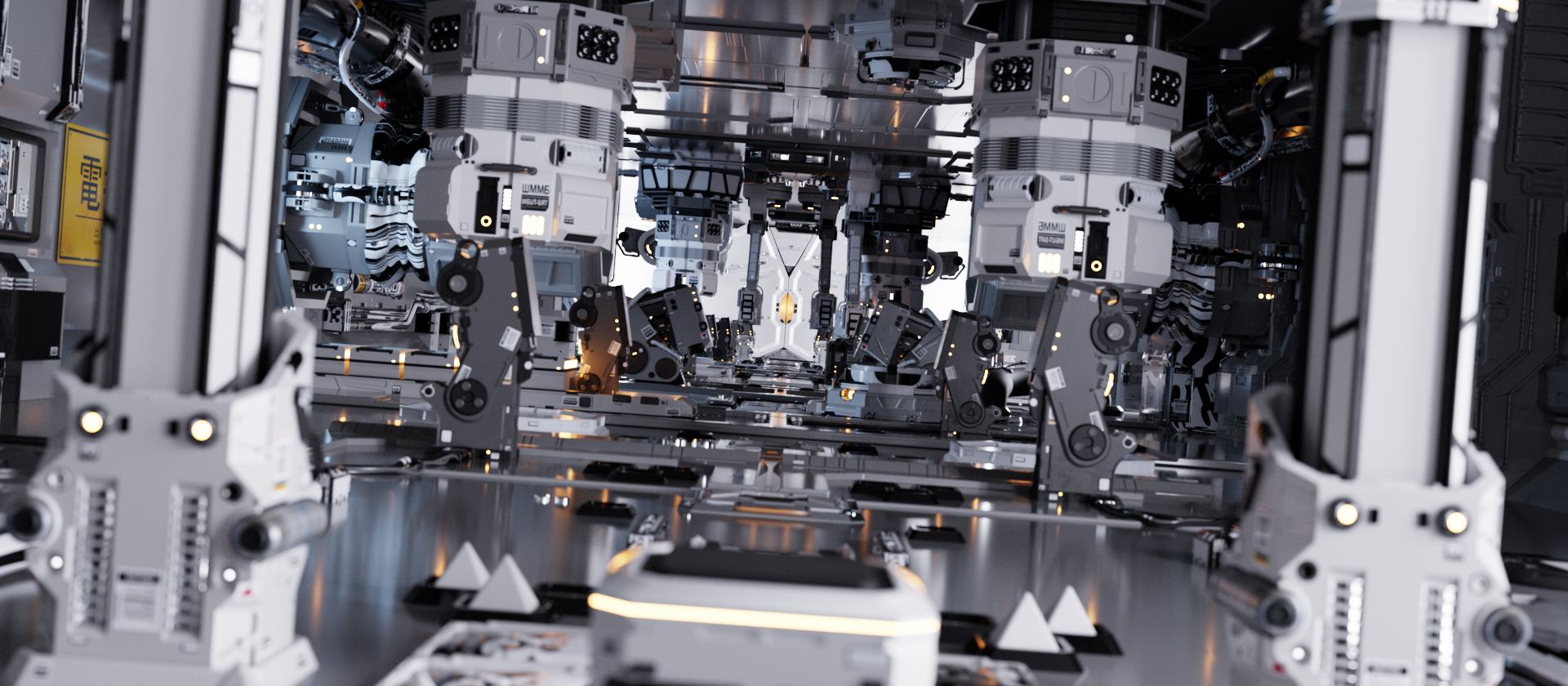
Of course, most scenes are made up of multiple objects. The brute-force approach would be to test the ray against each object in turn, choosing the minimum positive value of all intersections to find the closest intersection. This approach, while correct, is very slow, even for scenes of modest complexity. A better approach is to incorporate an acceleration structure that quickly rejects whole groups of objects during the ray intersection process. This ability to quickly cull irrelevant geometry means that ray tracing frequently runs in time, where is the number of pixels in the image and is the number of objects in the scene. ^† (Building the acceleration structure itself is necessarily at least O(n) time, however.) Thanks to the effectiveness of acceleration structures, it is possible to render highly complex scenes like the one shown in Figure 1.4 in reasonable amounts of time.

pbrt’s geometric interface and implementations of it for a variety of shapes are described in Chapter 6, and the acceleration interface and implementations are shown in Chapter 7.

1.2.3 Light Distribution

The ray–object intersection stage gives us a point to be shaded and some information about the local geometry at that point. Recall that our eventual goal is to find the amount of light leaving this point in the direction of the camera. To do this, we need to know how much light is arriving at this point. This involves both the geometric and radiometric distribution of light in the scene. For very simple light sources (e.g., point lights), the geometric distribution of lighting is a simple matter of knowing the position of the lights. However, point lights do not exist in the real world, and so physically based lighting is often based on area light sources. This means that the light source is associated with a geometric object that emits illumination from its surface. However, we will use point lights in this section to illustrate the components of light distribution; a more rigorous discussion of light measurement and distribution is the topic of Chapters 4 and 12.

We frequently would like to know the amount of light power being deposited on the differential area surrounding the intersection point (Figure 1.5). We will assume that the point light source has some power associated with it and that it radiates light equally in all directions. This means that the power per area on a unit sphere surrounding the light is . (These measurements will be explained and formalized in Section 4.1.)

If we consider two such spheres (Figure 1.6), it is clear that the power per area at a point on the larger sphere must be less than the power at a point on the smaller sphere because the same total power is distributed over a larger area. Specifically, the power per area arriving at a point on a sphere of radius is proportional to .

Furthermore, it can be shown that if the tiny surface patch d is tilted by an angle away from the vector from the surface point to the light, the amount of power deposited on d is proportional to . Putting this all together, the differential power per area d (the differential irradiance) is

Readers already familiar with basic lighting in computer graphics will notice two familiar laws encoded in this equation: the cosine falloff of light for tilted surfaces mentioned above, and the one-over--squared falloff of light with distance.

Scenes with multiple lights are easily handled because illumination is linear: the contribution of each light can be computed separately and summed to obtain the overall contribution. An implication of the linearity of light is that sophisticated algorithms can be applied to randomly sample lighting from only some of the light sources at each shaded point in the scene; this is the topic of Section 12.6. Figure 1.7 shows a scene with thousands of light sources rendered in this way.

1.2.4 Visibility

The lighting distribution described in the previous section ignores one very important component: shadows. Each light contributes illumination to the point being shaded only if the path from the point to the light’s position is unobstructed (Figure 1.8).

Fortunately, in a ray tracer it is easy to determine if the light is visible from the point being shaded. We simply construct a new ray whose origin is at the surface point and whose direction points toward the light. These special rays are called shadow rays. If we trace this ray through the environment, we can check to see whether any intersections are found between the ray’s origin and the light source by comparing the parametric value of any intersections found to the parametric value along the ray of the light source position. If there is no blocking object between the light and the surface, the light’s contribution is included.

1.2.5 Light Scattering at Surfaces

We are now able to compute two pieces of information that are vital for proper shading of a point: its location and the incident lighting. Now we need to determine how the incident lighting is scattered at the surface. Specifically, we are interested in the amount of light energy scattered back along the ray that we originally traced to find the intersection point, since that ray leads to the camera (Figure 1.9).

Each object in the scene provides a material, which is a description of its appearance properties at each point on the surface. This description is given by the bidirectional reflectance distribution function (BRDF). This function tells us how much energy is reflected from an incoming direction to an outgoing direction . We will write the BRDF at as . (By convention, directions are unit vectors.)

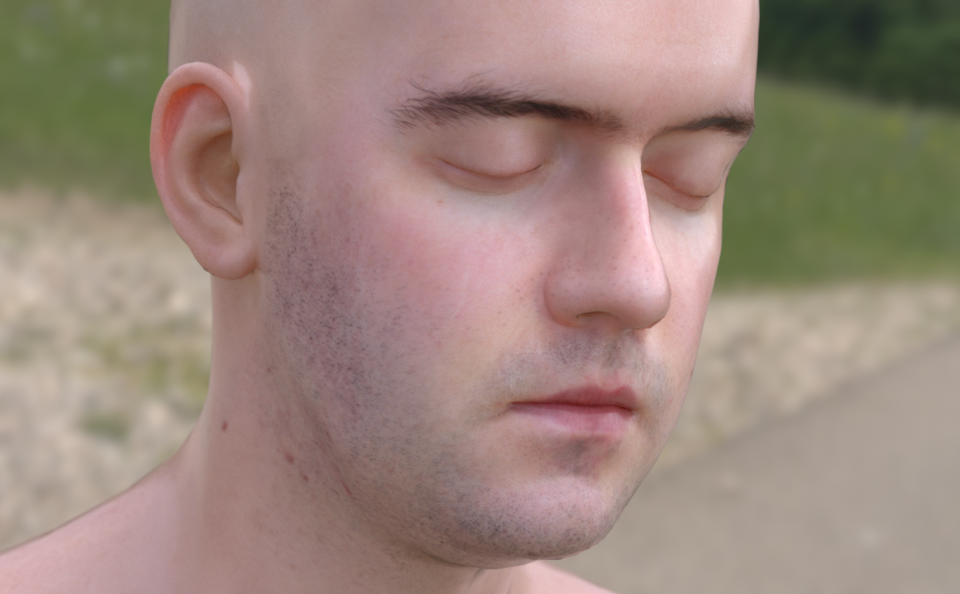
It is easy to generalize the notion of a BRDF to transmitted light (obtaining a BTDF) or to general scattering of light arriving from either side of the surface. A function that describes general scattering is called a bidirectional scattering distribution function (BSDF). pbrt supports a variety of BSDF models; they are described in Chapter 9. More complex yet is the bidirectional scattering surface reflectance distribution function (BSSRDF), which models light that exits a surface at a different point than it enters. This is necessary to reproduce translucent materials such as milk, marble, or skin. The BSSRDF is described in Figure 1.10 shows an image rendered by pbrt based on a model of a human head where scattering from the skin is modeled using a BSSRDF.

1.2.6 Indirect Light Transport

Turner Whitted’s original paper on ray tracing (1980) emphasized its recursive nature, which was the key that made it possible to include indirect specular reflection and transmission in rendered images. For example, if a ray from the camera hits a shiny object like a mirror, we can reflect the ray about the surface normal at the intersection point and recursively invoke the ray-tracing routine to find the light arriving at the point on the mirror, adding its contribution to the original camera ray. This same technique can be used to trace transmitted rays that intersect transparent objects. Many early ray-tracing examples showcased mirrors and glass balls (Figure 1.11) because these types of effects were difficult to capture with other rendering techniques.

In general, the amount of light that reaches the camera from a point on an object is given by the sum of light emitted by the object (if it is itself a light source) and the amount of reflected light. This idea is formalized by the light transport equation (also often known as the rendering equation), which measures light with respect to radiance, a radiometric unit that will be defined in Section 4.1. It says that the outgoing radiance from a point in direction is the emitted radiance at that point in that direction, , plus the incident radiance from all directions on the sphere around scaled by the BSDF and a cosine term:

We will show a more complete derivation of this equation in Sections 4.3.1 and 13.1.1. Solving this integral analytically is not possible except for the simplest of scenes, so we must either make simplifying assumptions or use numerical integration techniques.

Whitted’s ray-tracing algorithm simplifies this integral by ignoring incoming light from most directions and only evaluating for directions to light sources and for the directions of perfect reflection and refraction. In other words, it turns the integral into a sum over a small number of directions. In Section 1.3.6, we will see that simple random sampling of Equation (1.1) can create realistic images that include both complex lighting and complex surface scattering effects. Throughout the remainder of the book, we will show how using more sophisticated random sampling algorithms greatly improves the efficiency of this general approach.

1.2.7 Ray Propagation

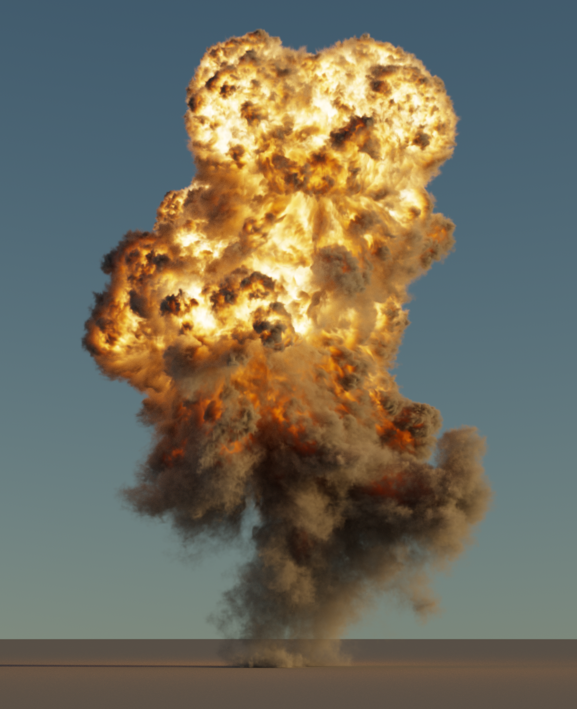
The discussion so far has assumed that rays are traveling through a vacuum. For example, when describing the distribution of light from a point source, we assumed that the light’s power was distributed equally on the surface of a sphere centered at the light without decreasing along the way. The presence of participating media such as smoke, fog, or dust can invalidate this assumption. These effects are important to simulate: a wide class of interesting phenomena can be described using participating media. Figure 1.12 shows an explosion rendered by pbrt. Less dramatically, almost all outdoor scenes are affected substantially by participating media. For example, Earth’s atmosphere causes objects that are farther away to appear less saturated.

There are two ways in which a participating medium can affect the light propagating along a ray. First, the medium can extinguish (or attenuate) light, either by absorbing it or by scattering it in a different direction. We can capture this effect by computing the transmittance  between the ray origin and the intersection point. The transmittance tells us how much of the light scattered at the intersection point makes it back to the ray origin.

A participating medium can also add to the light along a ray. This can happen either if the medium emits light (as with a flame) or if the medium scatters light from other directions back along the ray. We can find this quantity by numerically evaluating the volume light transport equation, in the same way we evaluated the light transport equation to find the amount of light reflected from a surface. We will leave the description of participating media and volume rendering until Chapters 11 and 14.