13.6 2D Sampling with Multidimensional Transformations

Suppose we have a 2D joint density function p left-parenthesis x comma y right-parenthesis that we wish to draw samples left-parenthesis upper X comma upper Y right-parenthesis from. Sometimes multidimensional densities are separable and can be expressed as the product of 1D densities—for example,

p left-parenthesis x comma y right-parenthesis equals p Subscript x Baseline left-parenthesis x right-parenthesis p Subscript y Baseline left-parenthesis y right-parenthesis comma

for some p Subscript x and p Subscript y . In this case, random variables left-parenthesis upper X comma upper Y right-parenthesis can be found by independently sampling upper X from p Subscript x and upper Y from p Subscript y . Many useful densities aren’t separable, however, so we will introduce the theory of how to sample from multidimensional distributions in the general case.

Given a 2D density function, the marginal density function p left-parenthesis x right-parenthesis is obtained by “integrating out” one of the dimensions:

p left-parenthesis x right-parenthesis equals integral p left-parenthesis x comma y right-parenthesis normal d y period

This can be thought of as the density function for upper X alone. More precisely, it is the average density for a particular x over all possible y values.

The conditional density function p left-parenthesis y vertical-bar x right-parenthesis is the density function for y given that some particular x has been chosen (it is read “ p of y given x ”):

p left-parenthesis y vertical-bar x right-parenthesis equals StartFraction p left-parenthesis x comma y right-parenthesis Over p left-parenthesis x right-parenthesis EndFraction period

The basic idea for 2D sampling from joint distributions is to first compute the marginal density to isolate one particular variable and draw a sample from that density using standard 1D techniques. Once that sample is drawn, one can then compute the conditional density function given that value and draw a sample from that distribution, again using standard 1D sampling techniques.

13.6.1 Uniformly Sampling a Hemisphere

As an example, consider the task of choosing a direction on the hemisphere uniformly with respect to solid angle. Remember that a uniform distribution means that the density function is a constant, so we know that p left-parenthesis omega right-parenthesis equals c . In conjunction with the fact that the density function must integrate to one over its domain, we have

integral Underscript script upper H squared Endscripts p left-parenthesis omega right-parenthesis normal d omega Subscript Baseline equals 1 right double arrow c integral Underscript script upper H squared Endscripts normal d omega Subscript Baseline equals 1 right double arrow c equals StartFraction 1 Over 2 pi EndFraction period

This tells us that p left-parenthesis omega right-parenthesis equals 1 slash left-parenthesis 2 pi right-parenthesis , or p left-parenthesis theta comma phi right-parenthesis equals sine theta slash left-parenthesis 2 pi right-parenthesis (using a result from the previous example about spherical coordinates). Note that this density function is separable. Nevertheless, we will use the marginal and conditional densities to illustrate the multidimensional sampling technique.

Consider sampling theta first. To do so, we need theta ’s marginal density function p left-parenthesis theta right-parenthesis :

p left-parenthesis theta right-parenthesis equals integral Subscript 0 Superscript 2 pi Baseline p left-parenthesis theta comma phi right-parenthesis normal d phi Subscript Baseline equals integral Subscript 0 Superscript 2 pi Baseline StartFraction sine theta Over 2 pi EndFraction normal d phi Subscript Baseline equals sine theta period

Now, compute the conditional density for phi :

p left-parenthesis phi vertical-bar theta right-parenthesis equals StartFraction p left-parenthesis theta comma phi right-parenthesis Over p left-parenthesis theta right-parenthesis EndFraction equals StartFraction 1 Over 2 pi EndFraction period

Notice that the density function for phi is itself uniform; this should make intuitive sense given the symmetry of the hemisphere. Now, we use the 1D inversion technique to sample each of these PDFs in turn:

StartLayout 1st Row 1st Column upper P left-parenthesis theta right-parenthesis 2nd Column equals integral Subscript 0 Superscript theta Baseline sine theta prime normal d theta Subscript Superscript prime Baseline equals 1 minus cosine theta 2nd Row 1st Column upper P left-parenthesis phi vertical-bar theta right-parenthesis 2nd Column equals integral Subscript 0 Superscript phi Baseline StartFraction 1 Over 2 pi EndFraction normal d phi Superscript prime Baseline equals StartFraction phi Over 2 pi EndFraction period EndLayout

Inverting these functions is straightforward, and here we can safely replace 1 minus xi Subscript with xi Subscript , giving

StartLayout 1st Row 1st Column theta 2nd Column equals cosine Superscript negative 1 Baseline xi 1 2nd Row 1st Column phi 2nd Column equals 2 pi xi 2 period EndLayout

Converting these back to Cartesian coordinates, we get the final sampling formulae:

StartLayout 1st Row 1st Column x 2nd Column equals sine theta cosine phi equals cosine left-parenthesis 2 pi xi 2 right-parenthesis StartRoot 1 minus xi 1 squared EndRoot 2nd Row 1st Column y 2nd Column equals sine theta sine phi equals sine left-parenthesis 2 pi xi 2 right-parenthesis StartRoot 1 minus xi 1 squared EndRoot 3rd Row 1st Column z 2nd Column equals cosine theta equals xi 1 period EndLayout

This sampling strategy is implemented in the following code. Two uniform random numbers are provided in u, and a vector on the hemisphere is returned.

<<Sampling Function Definitions>>+=  
Vector3f UniformSampleHemisphere(const Point2f &u) { Float z = u[0]; Float r = std::sqrt(std::max((Float)0, (Float)1. - z * z)); Float phi = 2 * Pi * u[1]; return Vector3f(r * std::cos(phi), r * std::sin(phi), z); }

For each sampling routine like this in pbrt, there is a corresponding function that returns the value of the PDF for a particular sample. For such functions, it is important to be clear which PDF is being evaluated—for example, for a direction on the hemisphere, we have already seen these densities expressed differently in terms of solid angle and in terms of left-parenthesis theta comma phi right-parenthesis . For hemispheres (and all other directional sampling), these functions return values with respect to solid angle. For the hemisphere, the solid angle PDF is a constant p left-parenthesis omega right-parenthesis equals 1 slash left-parenthesis 2 pi right-parenthesis .

<<Sampling Function Definitions>>+=  
Float UniformHemispherePdf() { return Inv2Pi; }

Sampling the full sphere uniformly over its area follows almost exactly the same derivation, which we omit here. The end result is

StartLayout 1st Row 1st Column x 2nd Column equals cosine left-parenthesis 2 pi xi 2 right-parenthesis StartRoot 1 minus z squared EndRoot equals cosine left-parenthesis 2 pi xi 2 right-parenthesis 2 StartRoot xi 1 left-parenthesis 1 minus xi 1 right-parenthesis EndRoot 2nd Row 1st Column y 2nd Column equals sine left-parenthesis 2 pi xi 2 right-parenthesis StartRoot 1 minus z squared EndRoot equals sine left-parenthesis 2 pi xi 2 right-parenthesis 2 StartRoot xi 1 left-parenthesis 1 minus xi 1 right-parenthesis EndRoot 3rd Row 1st Column z 2nd Column equals 1 minus 2 xi 1 period EndLayout

<<Sampling Function Definitions>>+=  
Vector3f UniformSampleSphere(const Point2f &u) { Float z = 1 - 2 * u[0]; Float r = std::sqrt(std::max((Float)0, (Float)1 - z * z)); Float phi = 2 * Pi * u[1]; return Vector3f(r * std::cos(phi), r * std::sin(phi), z); }

<<Sampling Function Definitions>>+=  
Float UniformSpherePdf() { return Inv4Pi; }

13.6.2 Sampling a Unit Disk

Although the disk seems a simpler shape to sample than the hemisphere, it can be trickier to sample uniformly because it has an incorrect intuitive solution. The wrong approach is the seemingly obvious one: r equals xi 1 comma theta equals 2 pi xi 2 . Although the resulting point is both random and inside the circle, it is not uniformly distributed; it actually clumps samples near the center of the circle. Figure 13.10(a) shows a plot of samples on the unit disk when this mapping was used for a set of uniform random samples left-parenthesis xi 1 comma xi 2 right-parenthesis . Figure 13.10(b) shows uniformly distributed samples resulting from the following correct approach.

Figure 13.10: (a) When the obvious but incorrect mapping of uniform random variables to points on the disk is used, the resulting distribution is not uniform and the samples are more likely to be near the center of the disk. (b) The correct mapping gives a uniform distribution of points.

Since we’re going to sample uniformly with respect to area, the PDF p left-parenthesis x comma y right-parenthesis must be a constant. By the normalization constraint, p left-parenthesis x comma y right-parenthesis equals 1 slash pi . If we transform into polar coordinates (see the example in Section 13.5.2), we have p left-parenthesis r comma theta right-parenthesis equals r slash pi . Now we compute the marginal and conditional densities as before:

StartLayout 1st Row 1st Column p left-parenthesis r right-parenthesis 2nd Column equals integral Subscript 0 Superscript 2 pi Baseline p left-parenthesis r comma theta right-parenthesis normal d theta Subscript Baseline equals 2 r 2nd Row 1st Column p left-parenthesis theta vertical-bar r right-parenthesis 2nd Column equals StartFraction p left-parenthesis r comma theta right-parenthesis Over p left-parenthesis r right-parenthesis EndFraction equals StartFraction 1 Over 2 pi EndFraction period EndLayout

As with the hemisphere case, the fact that p left-parenthesis theta vertical-bar r right-parenthesis is a constant should make sense because of the symmetry of the circle. Integrating and inverting to find upper P left-parenthesis r right-parenthesis , upper P Superscript negative 1 Baseline left-parenthesis r right-parenthesis , upper P left-parenthesis theta right-parenthesis , and upper P Superscript negative 1 Baseline left-parenthesis theta right-parenthesis , we can find that the correct solution to generate uniformly distributed samples on a disk is

StartLayout 1st Row 1st Column r 2nd Column equals StartRoot xi 1 EndRoot 2nd Row 1st Column theta 2nd Column equals 2 pi xi 2 period EndLayout

Taking the square root of xi 1 effectively pushes the samples back toward the edge of the disk, counteracting the clumping referred to earlier.

<<Sampling Function Definitions>>+=  
Point2f UniformSampleDisk(const Point2f &u) { Float r = std::sqrt(u[0]); Float theta = 2 * Pi * u[1]; return Point2f(r * std::cos(theta), r * std::sin(theta)); }

Although this mapping solves the problem at hand, it distorts areas on the disk; areas on the unit square are elongated and/or compressed when mapped to the disk (Figure 13.11). (Section 13.8.3 will discuss in more detail why this distortion is a disadvantage.)

Figure 13.11: The mapping from 2D random samples to points on the disk implemented in UniformSampleDisk() distorts areas substantially. Each section of the disk here has equal area and represents one-eighth of the unit square of uniform random samples in each direction. In general, we’d prefer a mapping that did a better job at mapping nearby left-parenthesis xi 1 comma xi 2 right-parenthesis values to nearby points on the disk.

A better approach is a “concentric” mapping from the unit square to the unit circle that avoids this problem. The concentric mapping takes points in the square left-bracket negative 1 comma 1 right-bracket squared to the unit disk by uniformly mapping concentric squares to concentric circles (Figure 13.12).

Figure 13.12: The concentric mapping maps squares to circles, giving a less distorted mapping than the first method shown for uniformly sampling points on the unit disk.

The mapping turns wedges of the square into slices of the disk. For example, points in the shaded area in Figure 13.12 are mapped to left-parenthesis r comma theta right-parenthesis  by

StartLayout 1st Row 1st Column r 2nd Column equals x 2nd Row 1st Column theta 2nd Column equals StartFraction y Over x EndFraction StartFraction pi Over 4 EndFraction period EndLayout

See Figure 13.13. The other seven wedges are handled analogously.

Figure 13.13: Triangular wedges of the square are mapped into left-parenthesis r comma theta right-parenthesis pairs in pie-shaped slices of the circle.

<<Sampling Function Definitions>>+=  
Point2f ConcentricSampleDisk(const Point2f &u) { <<Map uniform random numbers to left-bracket negative 1 comma 1 right-bracket squared >> 
Point2f uOffset = 2.f * u - Vector2f(1, 1);
<<Handle degeneracy at the origin>> 
if (uOffset.x == 0 && uOffset.y == 0) return Point2f(0, 0);
<<Apply concentric mapping to point>> 
Float theta, r; if (std::abs(uOffset.x) > std::abs(uOffset.y)) { r = uOffset.x; theta = PiOver4 * (uOffset.y / uOffset.x); } else { r = uOffset.y; theta = PiOver2 - PiOver4 * (uOffset.x / uOffset.y); } return r * Point2f(std::cos(theta), std::sin(theta));
}

<<Map uniform random numbers to left-bracket negative 1 comma 1 right-bracket squared >>= 
Point2f uOffset = 2.f * u - Vector2f(1, 1);

<<Handle degeneracy at the origin>>= 
if (uOffset.x == 0 && uOffset.y == 0) return Point2f(0, 0);

<<Apply concentric mapping to point>>= 
Float theta, r; if (std::abs(uOffset.x) > std::abs(uOffset.y)) { r = uOffset.x; theta = PiOver4 * (uOffset.y / uOffset.x); } else { r = uOffset.y; theta = PiOver2 - PiOver4 * (uOffset.x / uOffset.y); } return r * Point2f(std::cos(theta), std::sin(theta));

13.6.3 Cosine-Weighted Hemisphere Sampling

As we will see in Section 13.10, it is often useful to sample from a distribution that has a shape similar to that of the integrand being estimated. For example, because the scattering equation weights the product of the BSDF and the incident radiance with a cosine term, it is useful to have a method that generates directions that are more likely to be close to the top of the hemisphere, where the cosine term has a large value, than the bottom, where the cosine term is small.

Mathematically, this means that we would like to sample directions omega Subscript from a PDF

p left-parenthesis omega right-parenthesis proportional-to cosine theta period

Normalizing as usual,

StartLayout 1st Row 1st Column integral Underscript script upper H squared Endscripts p left-parenthesis omega Subscript Baseline right-parenthesis normal d omega Subscript 2nd Column equals 1 2nd Row 1st Column integral Subscript 0 Superscript 2 pi Baseline integral Subscript 0 Superscript StartFraction pi Over 2 EndFraction Baseline c cosine theta sine theta normal d theta Subscript Baseline normal d phi Subscript 2nd Column equals 1 3rd Row 1st Column c Baseline 2 pi integral Subscript 0 Superscript pi slash 2 Baseline cosine theta sine theta normal d theta Subscript 2nd Column equals 1 4th Row 1st Column c 2nd Column equals StartFraction 1 Over pi EndFraction EndLayout

so

p left-parenthesis theta comma phi right-parenthesis equals StartFraction 1 Over pi EndFraction cosine theta sine theta period

We could compute the marginal and conditional densities as before, but instead we can use a technique known as Malley’s method to generate these cosine-weighted points. The idea behind Malley’s method is that if we choose points uniformly from the unit disk and then generate directions by projecting the points on the disk up to the hemisphere above it, the resulting distribution of directions will have a cosine distribution (Figure 13.14).

Figure 13.14: Malley’s Method. To sample direction vectors from a cosine-weighted distribution, uniformly sample points on the unit disk and project them up to the unit hemisphere.

Why does this work? Let left-parenthesis r comma phi right-parenthesis be the polar coordinates of the point chosen on the disk (note that we’re using phi instead of the usual theta here). From our calculations before, we know that the joint density p left-parenthesis r comma phi right-parenthesis equals r slash pi gives the density of a point sampled on the disk.

Now, we map this to the hemisphere. The vertical projection gives sine theta equals r , which is easily seen from Figure 13.14. To complete the left-parenthesis r comma phi right-parenthesis equals left-parenthesis sine theta comma phi right-parenthesis right-arrow left-parenthesis theta comma phi right-parenthesis transformation, we need the determinant of the Jacobian

StartAbsoluteValue upper J Subscript upper T Baseline EndAbsoluteValue equals Start 2 By 2 Determinant 1st Row 1st Column cosine theta 2nd Column 0 2nd Row 1st Column 0 2nd Column 1 EndDeterminant equals cosine theta period

Therefore,

p left-parenthesis theta comma phi right-parenthesis equals StartAbsoluteValue upper J Subscript upper T Baseline EndAbsoluteValue p left-parenthesis r comma phi right-parenthesis equals cosine theta StartFraction r Over pi EndFraction equals left-parenthesis cosine theta sine theta right-parenthesis slash pi comma

which is exactly what we wanted! We have used the transformation method to prove that Malley’s method generates directions with a cosine-weighted distribution. Note that this technique works regardless of the method used to sample points from the circle, so we can use the earlier concentric mapping just as well as the simpler left-parenthesis r comma theta right-parenthesis equals left-parenthesis StartRoot xi 1 EndRoot comma 2 pi xi 2 right-parenthesis method.

<<Sampling Inline Functions>>+=  
inline Vector3f CosineSampleHemisphere(const Point2f &u) { Point2f d = ConcentricSampleDisk(u); Float z = std::sqrt(std::max((Float)0, 1 - d.x * d.x - d.y * d.y)); return Vector3f(d.x, d.y, z); }

Remember that all of the directional PDF evaluation routines in pbrt are defined with respect to solid angle, not spherical coordinates, so the PDF function returns a weight of cosine theta slash pi .

<<Sampling Inline Functions>>+=  
inline Float CosineHemispherePdf(Float cosTheta) { return cosTheta * InvPi; }

13.6.4 Sampling a Cone

For both area light sources based on Spheres as well as for the SpotLight, it’s useful to be able to uniformly sample rays in a cone of directions. Such distributions are separable in left-parenthesis theta comma phi right-parenthesis , with p left-parenthesis phi right-parenthesis equals 1 slash left-parenthesis 2 pi right-parenthesis and so we therefore need to derive a method to sample a direction theta uniformly over the cone of directions around a central direction up to the maximum angle of the beam, theta Subscript normal m normal a normal x . Incorporating the sine theta term from the measure on the unit sphere from Equation (5.5),

StartLayout 1st Row 1st Column 1 2nd Column equals c integral Subscript 0 Superscript theta Subscript normal m normal a normal x Baseline Baseline sine theta normal d theta Subscript Baseline 2nd Row 1st Column Blank 2nd Column equals c left-parenthesis 1 minus cosine theta Subscript normal m normal a normal x Baseline right-parenthesis period EndLayout

So p left-parenthesis theta right-parenthesis equals sine theta slash left-parenthesis 1 minus cosine theta Subscript normal m normal a normal x Baseline right-parenthesis and p left-parenthesis omega right-parenthesis equals 1 slash left-parenthesis 2 pi left-parenthesis 1 minus cosine theta Subscript normal m normal a normal x Baseline right-parenthesis right-parenthesis .

<<Sampling Function Definitions>>+=  
Float UniformConePdf(Float cosThetaMax) { return 1 / (2 * Pi * (1 - cosThetaMax)); }

The PDF can be integrated to find the CDF, and the sampling technique,

cosine theta equals left-parenthesis 1 minus xi Subscript Baseline right-parenthesis plus xi Subscript Baseline cosine theta Subscript normal m normal a normal x Baseline comma

follows. There are two UniformSampleCone() functions that implement this sampling technique: the first samples about the left-parenthesis 0 comma 0 comma 1 right-parenthesis axis, and the second (not shown here) takes three basis vectors for the coordinate system to be used where samples taken are with respect to the z axis of the given coordinate system.

<<Sampling Function Definitions>>+=  
Vector3f UniformSampleCone(const Point2f &u, Float cosThetaMax) { Float cosTheta = ((Float)1 - u[0]) + u[0] * cosThetaMax; Float sinTheta = std::sqrt((Float)1 - cosTheta * cosTheta); Float phi = u[1] * 2 * Pi; return Vector3f(std::cos(phi) * sinTheta, std::sin(phi) * sinTheta, cosTheta); }

13.6.5 Sampling a Triangle

Although uniformly sampling a triangle may seem like a simple task, it turns out to be more complex than the ones we’ve seen so far. To simplify the problem, we will assume we are sampling an isosceles right triangle of area one-half . The output of the sampling routine that we will derive will be barycentric coordinates, however, so the technique will actually work for any triangle despite this simplification. Figure 13.15 shows the shape to be sampled.

Figure 13.15: Sampling an Isosceles Right Triangle. Note that the equation of the hypotenuse is v equals 1 minus u .

We will denote the two barycentric coordinates here by left-parenthesis u comma v right-parenthesis . Since we are sampling with respect to area, we know that the PDF p left-parenthesis u comma v right-parenthesis must be a constant equal to the reciprocal of the shape’s area, one-half , so p left-parenthesis u comma v right-parenthesis equals 2 .

First, we find the marginal density p left-parenthesis u right-parenthesis :

p left-parenthesis u right-parenthesis equals integral Subscript 0 Superscript 1 minus u Baseline p left-parenthesis u comma v right-parenthesis normal d v equals 2 integral Subscript 0 Superscript 1 minus u Baseline normal d v equals 2 left-parenthesis 1 minus u right-parenthesis comma

and the conditional density p left-parenthesis v vertical-bar u right-parenthesis :

p left-parenthesis v vertical-bar u right-parenthesis equals StartFraction p left-parenthesis u comma v right-parenthesis Over p left-parenthesis u right-parenthesis EndFraction equals StartFraction 2 Over 2 left-parenthesis 1 minus u right-parenthesis EndFraction equals StartFraction 1 Over 1 minus u EndFraction period

The CDFs are, as always, found by integration:

StartLayout 1st Row 1st Column upper P left-parenthesis u right-parenthesis 2nd Column equals integral Subscript 0 Superscript u Baseline p left-parenthesis u prime right-parenthesis normal d u Superscript prime Baseline equals 2 u minus u squared 2nd Row 1st Column upper P left-parenthesis v right-parenthesis 2nd Column equals integral Subscript 0 Superscript v Baseline p left-parenthesis v prime vertical-bar u right-parenthesis normal d v Superscript prime Baseline equals StartFraction v Over 1 minus u EndFraction period EndLayout

Inverting these functions and assigning them to uniform random variables gives the final sampling strategy:

StartLayout 1st Row 1st Column u 2nd Column equals 1 minus StartRoot xi 1 EndRoot 2nd Row 1st Column v 2nd Column equals xi 2 StartRoot xi 1 EndRoot period EndLayout

Notice that the two variables in this case are not independent!

<<Sampling Function Definitions>>+=  
Point2f UniformSampleTriangle(const Point2f &u) { Float su0 = std::sqrt(u[0]); return Point2f(1 - su0, u[1] * su0); }

We won’t provide a PDF evaluation function for this sampling strategy since the PDF’s value is just one over the triangle’s area.

13.6.6 Sampling Cameras

Section 6.4.7 described the radiometry of the measurement that is performed by film in a realistic camera. For reference, the equation that gave joules arriving over an area of the sensor, Equation (6.7), is

upper J equals StartFraction 1 Over z squared EndFraction integral Underscript upper A Subscript normal p Baseline Endscripts integral Subscript t 0 Superscript t 1 Baseline integral Underscript upper A Subscript normal e Baseline Endscripts upper L Subscript normal i Baseline left-parenthesis normal p Subscript Baseline comma normal p prime comma t Superscript prime Baseline right-parenthesis StartAbsoluteValue cosine Superscript 4 Baseline theta EndAbsoluteValue normal d upper A Subscript normal e Baseline normal d t prime normal d upper A Subscript normal p Baseline comma

where the areas integrated over are the area of a pixel on the film, upper A Subscript normal p , and an area over the rear lens element that bounds the lens’s exit pupil, upper A Subscript normal e . The integration over the pixel in the film is handled by the Integrator and the Sampler, so here we’ll consider the estimate

StartFraction 1 Over z squared EndFraction integral Subscript t 0 Superscript t 1 Baseline integral Underscript upper A Subscript normal e Endscripts upper L Subscript normal i Baseline left-parenthesis normal p Subscript Baseline comma normal p prime comma t Superscript prime Baseline right-parenthesis StartAbsoluteValue cosine Superscript 4 Baseline theta EndAbsoluteValue normal d upper A Subscript normal e Baseline normal d t prime

for a fixed point on the film plane normal p Subscript .

Given a PDF for sampling a time and a PDF for sampling a point on the exit pupil, p left-parenthesis upper A Subscript normal e Baseline right-parenthesis , we have the estimator

StartFraction 1 Over z squared EndFraction StartFraction upper L Subscript normal i Baseline left-parenthesis normal p Subscript Baseline comma normal p prime comma t right-parenthesis StartAbsoluteValue cosine Superscript 4 Baseline theta EndAbsoluteValue Over p left-parenthesis t right-parenthesis p left-parenthesis upper A Subscript normal e Baseline right-parenthesis EndFraction period

For a uniformly sampled time value, p left-parenthesis t right-parenthesis equals 1 slash left-parenthesis t 1 minus t 0 right-parenthesis . The weighting factor that should be applied to the incident radiance function upper L Subscript normal i to compute an estimate of Equation (6.7) is then

StartFraction left-parenthesis t 1 minus t 0 right-parenthesis StartAbsoluteValue cosine Superscript 4 Baseline theta EndAbsoluteValue Over z squared p left-parenthesis upper A Subscript normal e Baseline right-parenthesis EndFraction period

Recall from Section 6.4.5 that points on the exit pupil were uniformly sampled within a 2D bounding box. Therefore, to compute p left-parenthesis upper A Subscript normal e Baseline right-parenthesis , we just need one over the area of this bounding box. Conveniently, RealisticCamera::SampleExitPupil() returns this value, which GenerateRay() stores in exitPupilBoundsArea.

The computation of this weight is implemented in <<Return weighting for RealisticCamera ray>>; we can now see that if the simpleWeighting member variable is true, then the RealisticCamera computes a modified version of this term that only accounts for the cosine Superscript 4 Baseline theta term. While the value it computes isn’t a useful physical quantity, this option gives images with pixel values that are closely related to the scene radiance (with vignetting), which is often convenient.

<<Return weighting for RealisticCamera ray>>= 
Float cosTheta = Normalize(rFilm.d).z; Float cos4Theta = (cosTheta * cosTheta) * (cosTheta * cosTheta); if (simpleWeighting) return cos4Theta; else return (shutterClose - shutterOpen) * (cos4Theta * exitPupilBoundsArea) / (LensRearZ() * LensRearZ());

13.6.7 Piecewise-Constant 2D Distributions

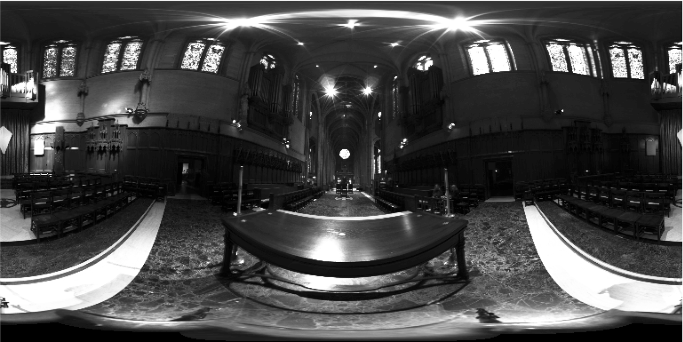
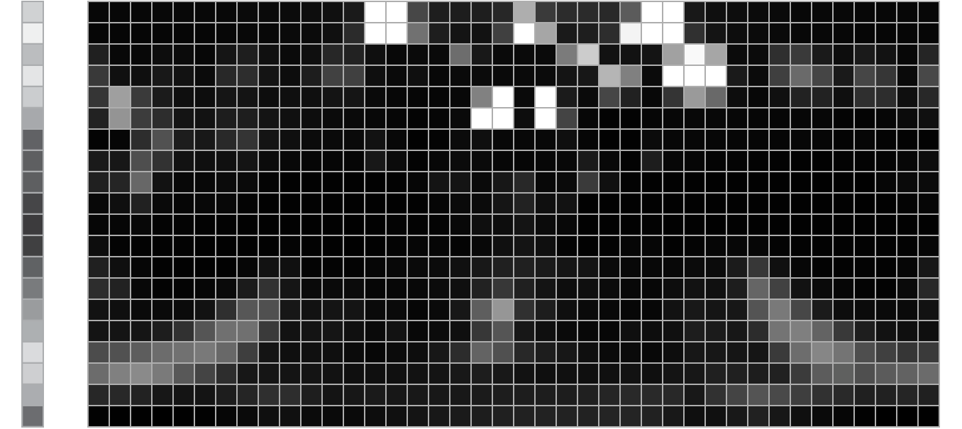
Our final example will show how to sample from discrete 2D distributions. We will consider the case of a 2D function defined over left-parenthesis u comma v right-parenthesis element-of left-bracket 0 comma 1 right-bracket squared by a 2D array of n Subscript u Baseline times n Subscript v sample values. This case is particularly useful for generating samples from distributions defined by texture maps and environment maps.

Consider a 2D function f left-parenthesis u comma v right-parenthesis defined by a set of n Subscript u Baseline times n Subscript v values f left-bracket u Subscript i Baseline comma v Subscript j Baseline right-bracket where u Subscript i Baseline element-of left-bracket 0 comma 1 comma ellipsis comma n Subscript u Baseline minus 1 right-bracket , v Subscript j Baseline element-of left-bracket 0 comma 1 comma ellipsis comma n Subscript v Baseline minus 1 right-bracket , and f left-bracket u Subscript i Baseline comma v Subscript j Baseline right-bracket give the constant value of f over the range left-bracket i slash n Subscript u Baseline comma left-parenthesis i plus 1 right-parenthesis slash n Subscript u Baseline right-parenthesis times left-bracket j slash n Subscript v Baseline comma left-parenthesis j plus 1 right-parenthesis slash n Subscript v Baseline right-parenthesis . Given continuous values left-parenthesis u comma v right-parenthesis , we will use left-parenthesis u overTilde comma v overTilde right-parenthesis to denote the corresponding discrete left-parenthesis u Subscript i Baseline comma v Subscript j Baseline right-parenthesis indices, with u overTilde equals left floor n Subscript u Baseline u right floor and v overTilde equals left floor n Subscript v Baseline v right floor so that f left-parenthesis u comma v right-parenthesis equals f left-bracket u overTilde comma v overTilde right-bracket .

Integrals of f are simple sums of f left-bracket u Subscript i Baseline comma v Subscript j Baseline right-bracket values, so that, for example, the integral of f over the domain is

upper I Subscript f Baseline equals integral integral f left-parenthesis u comma v right-parenthesis normal d u normal d v equals StartFraction 1 Over n Subscript u Baseline n Subscript v Baseline EndFraction sigma-summation Underscript i equals 0 Overscript n Subscript u Baseline minus 1 Endscripts sigma-summation Underscript j equals 0 Overscript n Subscript v Baseline minus 1 Endscripts f left-bracket u Subscript i Baseline comma v Subscript j Baseline right-bracket period

Using the definition of the PDF and the integral of f , we can find f ’s PDF,

p left-parenthesis u comma v right-parenthesis equals StartFraction f left-parenthesis u comma v right-parenthesis Over integral integral f left-parenthesis u comma v right-parenthesis normal d u normal d v EndFraction equals StartFraction f left-bracket u overTilde comma v overTilde right-bracket Over 1 slash left-parenthesis n Subscript u Baseline n Subscript v Baseline right-parenthesis sigma-summation Underscript i Endscripts sigma-summation Underscript j Endscripts f left-bracket u Subscript i Baseline comma v Subscript j Baseline right-bracket EndFraction period

Recalling Equation (13.11), the marginal density p left-parenthesis v right-parenthesis can be computed as a sum of f left-bracket u Subscript i Baseline comma v Subscript j Baseline right-bracket values

p left-parenthesis v right-parenthesis equals integral p left-parenthesis u comma v right-parenthesis normal d u equals StartFraction left-parenthesis 1 slash n Subscript u Baseline right-parenthesis sigma-summation Underscript i Endscripts f left-bracket u Subscript i Baseline comma v overTilde right-bracket Over upper I Subscript f Baseline EndFraction period

Because this function only depends on v overTilde , it is thus itself a piecewise constant 1D function, p left-bracket v overTilde right-bracket , defined by n Subscript v values. The 1D sampling machinery from Section 13.3.1 can be applied to sampling from its distribution.

Given a v sample, the conditional density p left-parenthesis u vertical-bar v right-parenthesis is then

p left-parenthesis u vertical-bar v right-parenthesis equals StartFraction p left-parenthesis u comma v right-parenthesis Over p left-parenthesis v right-parenthesis EndFraction equals StartFraction f left-bracket u overTilde comma v overTilde right-bracket slash upper I Subscript f Baseline Over p left-bracket v overTilde right-bracket EndFraction period

Note that, given a particular value of v overTilde , p left-bracket u overTilde vertical-bar v overTilde right-bracket is a piecewise-constant 1D function of u overTilde , that can be sampled with the usual 1D approach. There are n Subscript v such distinct 1D conditional densities, one for each possible value of v overTilde .

Putting this all together, the Distribution2D structure provides functionality similar to Distribution1D, except that it generates samples from piecewise-constant 2D distributions.

<<Sampling Declarations>>+= 
class Distribution2D { public: <<Distribution2D Public Methods>> 
Distribution2D(const Float *data, int nu, int nv); Point2f SampleContinuous(const Point2f &u, Float *pdf) const { Float pdfs[2]; int v; Float d1 = pMarginal->SampleContinuous(u[1], &pdfs[1], &v); Float d0 = pConditionalV[v]->SampleContinuous(u[0], &pdfs[0]); *pdf = pdfs[0] * pdfs[1]; return Point2f(d0, d1); } Float Pdf(const Point2f &p) const { int iu = Clamp(int(p[0] * pConditionalV[0]->Count()), 0, pConditionalV[0]->Count() - 1); int iv = Clamp(int(p[1] * pMarginal->Count()), 0, pMarginal->Count() - 1); return pConditionalV[iv]->func[iu] / pMarginal->funcInt; }
private: <<Distribution2D Private Data>> 
std::vector<std::unique_ptr<Distribution1D>> pConditionalV; std::unique_ptr<Distribution1D> pMarginal;
};

The constructor has two tasks. First, it computes a 1D conditional sampling density p left-bracket u overTilde vertical-bar v overTilde right-bracket for each of the n Subscript v individual v overTilde values using Equation (13.14). It then computes the marginal sampling density p left-bracket v overTilde right-bracket with Equation (13.13).

<<Sampling Function Definitions>>+= 
Distribution2D::Distribution2D(const Float *func, int nu, int nv) { for (int v = 0; v < nv; ++v) { <<Compute conditional sampling distribution for v overTilde >> 
pConditionalV.emplace_back(new Distribution1D(&func[v * nu], nu));
} <<Compute marginal sampling distribution p left-bracket v overTilde right-bracket >> 
std::vector<Float> marginalFunc; for (int v = 0; v < nv; ++v) marginalFunc.push_back(pConditionalV[v]->funcInt); pMarginal.reset(new Distribution1D(&marginalFunc[0], nv));
}

Distribution1D can directly compute the p left-bracket u overTilde vertical-bar v overTilde right-bracket distributions from a pointer to each of the n Subscript v rows of n Subscript u function values, since they’re laid out linearly in memory. The upper I Subscript f and p left-bracket v overTilde right-bracket terms from Equation (13.14) don’t need to be included in the values passed to Distribution1D, since they have the same value for all of the n Subscript u values and are thus just a constant scale that doesn’t affect the normalized distribution that Distribution1D computes.

<<Compute conditional sampling distribution for v overTilde >>= 
pConditionalV.emplace_back(new Distribution1D(&func[v * nu], nu));

<<Distribution2D Private Data>>= 
std::vector<std::unique_ptr<Distribution1D>> pConditionalV;

Given the conditional densities for each v overTilde value, we can find the 1D marginal density for sampling each v overTilde value, p left-bracket v overTilde right-bracket . The Distribution1D class stores the integral of the piecewise-constant function it represents in its funcInt member variable, so it’s just necessary to copy these values to the marginalFunc buffer so they’re stored linearly in memory for the Distribution1D constructor.

<<Compute marginal sampling distribution p left-bracket v overTilde right-bracket >>= 
std::vector<Float> marginalFunc; for (int v = 0; v < nv; ++v) marginalFunc.push_back(pConditionalV[v]->funcInt); pMarginal.reset(new Distribution1D(&marginalFunc[0], nv));

<<Distribution2D Private Data>>+= 
std::unique_ptr<Distribution1D> pMarginal;

As described previously, in order to sample from the 2D distribution, first a sample is drawn from the p left-bracket v overTilde right-bracket marginal distribution in order to find the v coordinate of the sample. The offset of the sampled function value gives the integer v overTilde value that determines which of the precomputed conditional distributions should be used for sampling the u value. Figure 13.16 illustrates this idea using a low-resolution image as an example.

Figure 13.16: The Piecewise-Constant Sampling Distribution for a High-Dynamic-Range Environment Map. (first) The original environment map, (second) a low-resolution version of the marginal density function p left-bracket ModifyingAbove v With caret right-bracket and the conditional distributions for rows of the image. First the marginal 1D distribution is used to select a v value, giving a row of the image to sample. Rows with bright pixels are more likely to be sampled. Then, given a row, a value u is sampled from that row’s 1D distribution. (Grace Cathedral environment map courtesy of Paul Debevec.)

<<Distribution2D Public Methods>>= 
Point2f SampleContinuous(const Point2f &u, Float *pdf) const { Float pdfs[2]; int v; Float d1 = pMarginal->SampleContinuous(u[1], &pdfs[1], &v); Float d0 = pConditionalV[v]->SampleContinuous(u[0], &pdfs[0]); *pdf = pdfs[0] * pdfs[1]; return Point2f(d0, d1); }

The value of the PDF for a given sample value is computed as the product of the conditional and marginal PDFs for sampling it from the distribution.

<<Distribution2D Public Methods>>+= 
Float Pdf(const Point2f &p) const { int iu = Clamp(int(p[0] * pConditionalV[0]->Count()), 0, pConditionalV[0]->Count() - 1); int iv = Clamp(int(p[1] * pMarginal->Count()), 0, pMarginal->Count() - 1); return pConditionalV[iv]->func[iu] / pMarginal->funcInt; }