13.2 Path Tracing
Now that we have derived the path integral form of the light transport equation, we will show how it can be used to derive the path-tracing light transport algorithm and will present a path-tracing integrator. Figure 13.4 compares images of a scene rendered with different numbers of pixel samples using the path-tracing integrator. In general, hundreds or thousands of samples per pixel may be necessary for high-quality results.
Path tracing was the first general-purpose unbiased Monte Carlo light transport algorithm used in graphics. Kajiya (1986) introduced it in the same paper that first described the light transport equation. Path tracing incrementally generates paths of scattering events starting at the camera and ending at light sources in the scene.
Although it is slightly easier to derive path tracing directly from the basic light transport equation, we will instead approach it from the path integral form, which helps build understanding of the path integral equation and makes the generalization to bidirectional path sampling algorithms easier to understand.
13.2.1 Overview
Given the path integral form of the LTE, we would like to estimate the value of the exitant radiance from the camera ray’s intersection point ,
for a given camera ray from that first intersects the scene at . We have two problems that must be solved in order to compute this estimate:
- How do we estimate the value of the sum of the infinite number of terms with a finite amount of computation?
- Given a particular term, how do we generate one or more paths in order to compute a Monte Carlo estimate of its multidimensional integral?
For path tracing, we can take advantage of the fact that for physically valid scenes, paths with more vertices scatter less light than paths with fewer vertices overall (this is not necessarily true for any particular pair of paths, just in the aggregate). This is a natural consequence of conservation of energy in BSDFs. Therefore, we will always estimate the first few terms and will then start to apply Russian roulette to stop sampling after a finite number of terms without introducing bias. (Recall that Section 2.2.4 showed how to use Russian roulette to probabilistically stop computing terms in a sum as long as the terms that are not skipped are reweighted appropriately.) For example, if we always computed estimates of , , and but stopped without computing more terms with probability , then an unbiased estimate of the sum would be
Using Russian roulette in this way does not solve the problem of needing to evaluate an infinite sum but has pushed it a bit farther out.
If we take this idea a step further and instead randomly consider terminating evaluation of the sum at each term with probability ,
we will eventually stop continued evaluation of the sum. Yet, because for any particular value of there is greater than zero probability of evaluating the term and because it will be weighted appropriately if we do evaluate it, the final result is an unbiased estimate of the sum.
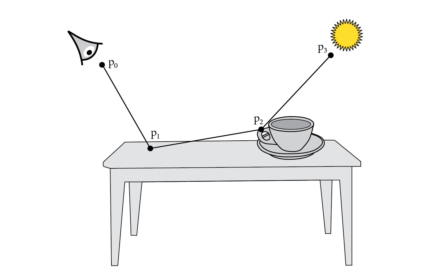
13.2.2 Path Sampling
Given this method for evaluating only a finite number of terms of the infinite sum, we also need a way to estimate the contribution of a particular term . We need vertices to specify the path, where the last vertex is on a light source and the first vertex is a point on the camera film or lens (Figure 13.5). Looking at the form of , a multiple integral over surface area of objects in the scene, the most natural thing to do is to sample vertices according to the surface area of objects in the scene, such that all points on surfaces in the scene are sampled with equal probability. (We do not actually use this approach in the integrator implementations in this chapter for reasons that will be described later, but this sampling technique could possibly be used to improve the efficiency of our basic implementation and helps to clarify the meaning of the path integral LTE.)
With this sampling approach, we might define a discrete probability over the objects in the scene. If each has surface area , then the probability of sampling a path vertex on the surface of the th object should be
Then, given a method to sample a point on the th object with uniform probability, the probability density function (PDF) for sampling any particular point on object is . Thus, the overall probability density for sampling the point is
and all samples have the same PDF value:
It is reassuring that they all have the same weight, since our intent was to choose among all points on surfaces in the scene with equal probability.
Given the set of vertices sampled in this manner, we can then sample the last vertex on a light source in the scene, defining its PDF in the same way. Although we could use the same technique used for sampling path vertices to sample points on lights, this would usually lead to high variance, since for all the paths where was not on the surface of an emitter, the path would have zero value. The expected value would still be the correct value of the integral, but convergence would be extremely slow. A better approach is to sample over the areas of only the emitting objects with probabilities updated accordingly. Given a complete path, we have all the information we need to compute the estimate of ; it is just a matter of evaluating each of the terms.
It is easy to be more creative about how we set the sampling probabilities with this general approach. For example, if we knew that indirect illumination from a few objects contributed to most of the lighting in the scene, we could assign a higher probability to generating path vertices on those objects, updating the sample weights appropriately.
However, there are two interrelated problems with sampling paths in this manner. The first can lead to high variance, while the second can lead to incorrect results. The first problem is that many of the paths will have no contribution if they have pairs of adjacent vertices that are not mutually visible. Consider applying this area sampling method in a complex building model: adjacent vertices in the path will almost always have a wall or two between them, giving no contribution for the path and high variance in the estimate.
The second problem is that if the integrand has delta functions in it (e.g., a point light source or a perfect specular BSDF), this sampling technique will never be able to choose path vertices such that the delta distributions are nonzero. Even if there are no delta distributions, as the BSDFs become increasingly glossy almost all the paths will have low contributions since the points in will cause the BSDF to have a small or zero value, and again we will suffer from high variance.
13.2.3 Incremental Path Construction
A solution that solves both of these problems is to construct the path incrementally, starting from the vertex at the camera . At each vertex, the BSDF is sampled to generate a new direction; the next vertex is found by tracing a ray from in the sampled direction and finding the closest intersection. We are effectively trying to find a path with a large overall contribution by making a series of choices that find directions with important local contributions. While one can imagine situations where this approach could be ineffective, it is generally a good strategy.
Because this approach constructs the path by sampling BSDFs according to solid angle, and because the path integral LTE is an integral over surface area in the scene, we need to apply the correction to convert from the probability density according to solid angle to a density according to area (Section 4.2). If is the normalized direction sampled at , it is:
This correction causes all the factors of the corresponding geometric function to cancel out of except for the term. Furthermore, we already know that and must be mutually visible since we traced a ray to find , so the visibility term is trivially equal to 1. An alternative way to think about this is that ray tracing provides an operation to importance sample the visibility component of .
With path tracing, the last vertex of the path, which is on the surface of a light source, gets special treatment. Rather than being sampled incrementally, it is sampled from a distribution that is just over the surfaces of the lights. (Sampling the last vertex in this way is often referred to as next event estimation (NEE), after a Monte Carlo technique with that name.) For now we will assume there is such a sampling distribution over the emitters, though in Section 13.4 we will see that a more effective estimator can be constructed using multiple importance sampling.
With this approach, the value of the Monte Carlo estimate for a path is
Because this sampling scheme reuses vertices of the path of length (except the vertex on the emitter) when constructing the path of length , it does introduce correlation among the terms. This does not affect the unbiasedness of the Monte Carlo estimator, however. In practice this correlation is more than made up for by the improved efficiency from tracing fewer rays than would be necessary to make the terms independent.
Relationship to the RandomWalkIntegrator
With this derivation of the foundations of path tracing complete, the implementation of the RandomWalkIntegrator from Chapter 1 can now be understood more formally: at each path vertex, uniform spherical sampling is used for the distribution —and hence the division by , corresponding to the uniform spherical PDF. The factor in parentheses in Equation (13.7) is effectively computed via the product of beta values through recursive calls to RandomWalkIntegrator::LiRandomWalk(). Emissive surfaces contribute to the radiance estimate whenever a randomly sampled path hits a surface with a nonzero ; because directions are sampled with respect to solid angle, the factor in Equation (13.7) is not over emissive geometry but is the uniform directional probability . Most of the remaining factor then cancels out due to the change of variables from integrating over area to integrating over solid angle.