15.4 Sampling Subsurface Reflection Functions

We’ll now implement techniques to sample the subsurface scattering equation introduced in Section 5.6.2, building on the BSSRDF interface introduced in Section 11.4. Our task is to estimate

Figure 15.6 suggests the complexity of evaluating the integral. To compute the standard Monte Carlo estimate of this equation given a point at which to compute outgoing radiance, we need a technique to sample points on the surface and to compute the incident radiance at these points, as well as an efficient way to compute the specific value of the BSSRDF for each sampled point and incident direction.

The VolPathIntegrator could be used to evaluate the BSSRDF: given a pair of points on the surface and a pair of directions, the integrator can be used to compute the fraction of incident light from direction at the point that exits the object at the point in direction by following light-carrying paths through the multiple scattering events in the medium. Beyond standard path-tracing or bidirectional path-tracing techniques, many other light transport algorithms are applicable to this task.

However, many translucent objects are characterized by having very high albedos, which are not efficiently handled by classic approaches. For example, Jensen et al. (2001b) measured the scattering properties of skim milk and found an albedo of . When essentially all of the light is scattered at each interaction in the medium and almost none of it is absorbed, light easily travels far from where it first enters the medium. Hundreds or even thousands of scattering events must be considered to compute an accurate result; given the high albedo of milk, after 100 scattering events, of the incident light is still carried by a path, after 500 scattering events, and still after 1000.

BSSRDF class implementations represent the aggregate scattering behavior of these sorts of media, making it possible to render them fairly efficiently. Figure 15.7 shows an example of the dragon model rendered with a BSSRDF. The main sampling operation that must be provided by implementations of the BSSRDF interface, BSSRDF::Sample_S(), determines the surface position where a ray re-emerges following internal scattering.

The value of the BSSRDF for the two points and directions is returned directly, and the associated surface interaction record and probability density are returned via the si and pdf parameters. Two samples must be provided: a 1D sample for discrete sampling decisions (e.g., choosing a specific spectral channel of the profile) and a 2D sample that is mapped onto si. As we will see shortly, it’s useful for BSSRDF implementations to be able to trace rays against the scene geometry to find si, so the scene is also provided as an argument.

15.4.1 Sampling the SeparableBSSRDF

Recall the simplifying assumption introduced in Section 11.4.1, which factored the BSSRDF into spatial and directional components that can be sampled independently from one another. Specifically, Equation (11.6) defined as a product of a single spatial term and a pair of directional terms related to the incident and outgoing directions.

The spatial term was further simplified to a radial profile function :

We will now explain how each of these factors is handled by the SeparableBSSRDF’s sampling routines. This class implements an abstract sampling interface that works for any radial profile function . The TabulatedBSSRDF class, discussed in Section 15.4.2, derives from SeparableBSSRDF and provides a specific tabulated representation of this profile with support for efficient evaluation and exact importance sampling.

Returning to Equation (15.14), if we assume that the BSSRDF is only sampled for rays that are transmitted through the surface boundary, where transmission is selected with probability , then nothing needs to be done for the part here. (This is the case for the fragment <<Account for subsurface scattering, if applicable>>.) This is a reasonable expectation to place on calling code, as this approach gives good Monte Carlo efficiency.

This leaves the and terms—the former is handled by a call to SeparableBSSRDF::Sample_Sp() (to be discussed shortly), which returns the position si.

If sampling a position is successful, the method initializes si->bsdf with an instance of the class SeparableBSSRDFAdapter, which represents the directional term as a BxDF. Although this BxDF does not truly depend on the outgoing direction si->wo, we still need to initialize it with a dummy direction.

The SeparableBSSRDFAdapter class is a thin wrapper around SeparableBSSRDF::Sw(). Recall that from Equation (11.7) was defined as a diffuse-like term scaled by the normalized Fresnel transmission. For this reason, the SeparableBSSRDFAdapter classifies itself as BSDF_DIFFUSE and just uses the default cosine-weighted sampling routine provided by BxDF::Sample_f().

Similar to refractive BSDFs, a scaling factor related to the light transport mode must be applied to the value the f() method returns for the term. This issue is discussed in more detail in Section 16.1, and the fragment that applies this scaling, <<Update BSSRDF transmission term to account for adjoint light transport>>, is defined there.

To sample the spatial component , we need a way of mapping a 2D distribution function onto an arbitrary surface using a parameterization of the surface in the neighborhood of the outgoing position. A conceptually straightforward way to obtain such a parameterization is by means of geodesics, but finding and evaluating them is non-trivial and requires significant implementation effort for each shape that is supported. We use a much simpler approach that uses ray tracing to map the radial profile onto the scene geometry.

Figure 15.8 illustrates the basic idea: the position and associated normal define a planar approximation to the surface. Using 2D polar coordinates, we first sample an azimuth and a radius value centered around and then map this position onto the actual surface by intersecting an offset perpendicular ray with the primitive, producing the position . The SeparableBSSRDF class only supports radially symmetric profile functions; hence is drawn from a uniform distribution on , and is distributed according to the radial profile function .

There are still several difficulties with this basic approach:

• The radial profile is not necessarily uniform across wavelengths—in practice, the mean free path can differ by orders of magnitude between different spectral channels.
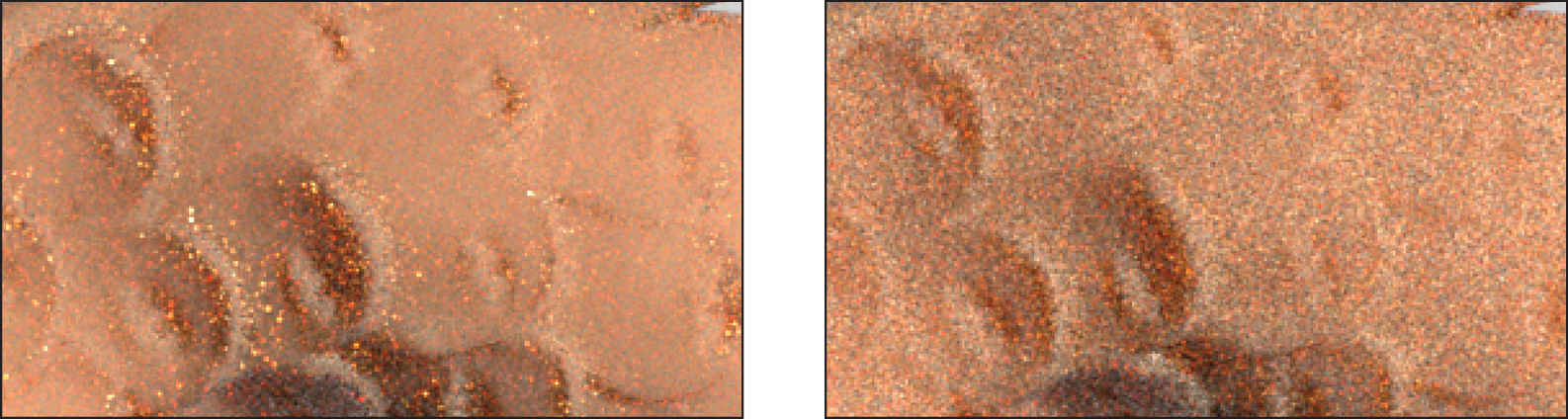
• If the surface geometry is poorly approximated by a plane and , where is the surface normal at , the probe rays will hit the surface at a grazing angle so that positions with comparatively high values of may be sampled with too low a probability. The result is high variance in renderings (Figure 15.9).
• Finally, the probe ray may intersect multiple surface locations along its length, all of which may contribute to reflected radiance.

The first two problems can be addressed with a familiar approach; namely, by introducing additional tailored sampling distributions and combining them using multiple importance sampling. The third will be addressed shortly.

We use a different sampling technique per wavelength to deal with spectral variation, and each technique is additionally replicated three times with different projection axes given by the basis vectors of a local frame, resulting in a total of 3 * Spectrum::nSamples sampling techniques. This ensures that every point where takes on non-negligible values is intersected with a reasonable probability. This combination of techniques is implemented in SeparableBSSRDF::Sample_Sp().

We begin by choosing a projection axis. Note that when the surface is close to planar, projecting along the normal SeparableBSSRDF::ns is clearly the best sampling strategy, as probe rays along the other two axes are likely to miss the surface. We therefore allocate a fairly large portion (50%) of the sample budget to perpendicular rays. The other half is equally shared between tangential projections along SeparableBSSRDF::ss and SeparableBSSRDF::ts. The three axes of the chosen coordinate system are stored in vx, vy, and vz, and follow our usual convention of measuring angles in spherical coordinates with respect to the axis.

After this discrete sampling operation, we scale and offset u1 so that additional sampling operations can reuse it as a uniform variate.

The fragments for the other two axes are similar and therefore not included here.

Next, we uniformly choose a spectral channel and re-scale u1 once more.

The 2D profile sampling operation is then carried out in polar coordinates using the SeparableBSSRDF::Sample_Sr() method. This method returns a negative radius to indicate a failure (e.g., when there is no scattering from channel ch); the implementation here returns a BSSRDF value of 0 in this case.

Both the radius sampling method SeparableBSSRDF::Sample_Sr() and its associated density function SeparableBSSRDF::Pdf_Sr() are declared as pure virtual functions; an implementation for TabulatedBSSRDF is presented in the next section.

Because the profile falls off fairly quickly, we are not interested in positions that are too far ^† away from . In order to reduce the computational expense of the ray-tracing step, the probe ray is clamped to a sphere of radius around . Another call to SeparableBSSRDF::Sample_Sr() is used to determine . Assuming that this function implements a perfect importance sampling scheme based on the inversion method (Section 13.3.1), Sample_Sr() maps a sample value to the radius of a sphere containing a fraction of the scattered energy.

Here, we set so that the sphere from Figure 15.8 contains 99.9% of the scattered energy. When lies outside of , sampling fails—this helps to keep the probe rays short, which significantly improves the run-time performance. Given and , the length of the intersection of the probe ray with the sphere of radius is

(See Figure 15.10.)

Given the sampled polar coordinate value, we can compute the world space origin of a ray that lies on the boundary of the sphere and a target point, pTarget, where it exits the sphere.

In practice, there could be more than just one intersection along the probe ray, and we want to collect all of them here. We’ll create a linked list of all of the found interactions.

IntersectionChain lets us maintain this list. Once again, the MemoryArena makes it possible to efficiently perform allocations, here for the list nodes.

We now start by finding intersections along the segment within the sphere. The list’s tail node’s SurfaceInteraction is initialized with each intersection’s information, and base Interaction is updated so that the next ray can be spawned on the other side of the intersected surface. (See Figure 15.11.)

When tracing rays to sample nearby points on the surface of the primitive, it’s important to ignore any intersections on other primitives in the scene. (There is an implicit assumption that scattering between primitives will be handled by the integrator, and the BSSRDF should be limited to account for single primitives’ scattering.) The implementation here uses equality of Material pointers as a proxy to determine if an intersection is on the same primitive. Valid intersections are appended to the chain, and the variable nFound records their total count when the loop terminates.

With the set of intersections at hand, we must now choose one of them, as Sample_Sp() can only return a single position . The following fragment uses the variable u1 one last time to pick one of the list entries with uniform probability.

Finally, we can call SeparableBSSRDF::Pdf_Sp() (to be defined shortly) to evaluate the combined PDF that takes all of the sampling strategies into account. The probability it returns is divided by nFound to account for the discrete probability of selecting pi from the IntersectionChain. Finally, the value of is returned.

SeparableBSSRDF::Pdf_Sp() returns the probability per unit area of sampling the position pi with the total of 3 * Spectrum::nSamples sampling techniques available to SeparableBSSRDF::Sample_Sp().

First, nLocal is initialized with the surface normal at and dLocal with the difference vector , both expressed using local coordinates at .

To determine the combined PDF, we must query the probability of sampling a radial profile radius matching the pair for each technique. This radius is measured in 2D and thus depends on the chosen projection axis (Figure 15.12). The rProj variable records radii for projections perpendicular to ss, ts, and ns.

The remainder of the implementation simply loops over all combinations of spectral channels and projection axes and sums up the product of the probability of selecting each technique and its area density under projection onto the surface at .

The alert reader may have noticed a slight inconsistency in the above definitions: the probability of choosing one of several (nFound) intersections in SeparableBSSRDF::Sample_Sp() should really have been part of the density function computed in the SeparableBSSRDF::Pdf_Sp() method rather than the ad hoc division that occurs in the fragment <<Compute sample PDF and return the spatial BSSRDF term >>. In practice, the number of detected intersections varies with respect of the projection axis and spectral channel; correctly accounting for this in the PDF computation requires counting the number of intersections along each of a total of 3 * Spectrum::nSamples probe rays for every sample! We neglect this issue, trading a more efficient implementation for a small amount of bias.

15.4.2 Sampling the TabulatedBSSRDF

The previous section completed the discussion of BSSRDF sampling with the exception of the Pdf_Sr() and Sample_Sr() methods that were declared as pure virtual functions in the SeparableBSSRDF interface. The TabulatedBSSRDF subclass implements this missing functionality.

The TabulatedBSSRDF::Sample_Sr() method samples radius values proportional to the radial profile function . Recall from Section 11.4.2 that the profile has an implicit dependence on the albedo at the current surface position and that the TabulatedBSSRDF provides interpolated evaluations of using 2D tensor product spline basis functions. TabulatedBSSRDF::Sample_Sr() then determines the albedo for the given spectral channel ch and draws samples proportional to the remaining 1D function . Sample generation fails if there is neither scattering nor absorption on channel ch (this case is indicated by returning a negative radius).

As in Section 11.4.2, there is a considerable amount of overlap with the FourierBSDF implementation. The sampling operation here actually reduces to a single call to SampleCatmullRom2D(), which was previously used in FourierBSDF::Sample_f().

Recall that this function depends on a precomputed CDF array, which is initialized when the BSSRDFTable is created.

The Pdf_Sr() method returns the PDF of samples obtained via Sample_Sr(). It evaluates the profile function divided by the normalizing constant defined in Equation (11.11).

The beginning is analogous to the spline evaluation code in TabulatedBSSRDF::Sr(). The fragment <<Compute spline weights to interpolate BSSRDF density on channel ch>> matches <<Compute spline weights to interpolate BSSRDF on channel ch>> in that method except that this method immediately returns zero if the optical radius is outside the range represented by the spline.

The remainder of the implementation is very similar to fragment <<Set BSSRDF value Sr[ch] using tensor spline interpolation>> except that here, we also interpolate from the tabulation and include it in the division at the end.

15.4.3 Subsurface Scattering in the Path Tracer

We now have the capability to apply Monte Carlo integration to the generalized scattering equation, (5.11), from Section 5.6.2. We will compute estimates of the form

where represents incident direct radiance and is incident indirect radiance. The sample is generated in two steps. First, given and , a call to BSSRDF::Sample_S() returns a position whose distribution is similar to the marginal distribution of with respect to .

Next, we sample the incident direction . Recall that the BSSRDF::Sample_S() interface intentionally keeps these two steps apart: instead of generating both and at the same time, it returns a special BSDF instance via the bsdf field of si that is used for the direction sampling step. No generality is lost with such an approach: the returned BSDF can be completely arbitrary and is explicitly allowed to depend on information computed within BSSRDF::Sample_S(). The benefit is that we can re-use a considerable amount of existing infrastructure for computing product integrals of a BSDF and .

The PathIntegrator’s <<Find next path vertex and accumulate contribution>> fragment invokes the following code to compute this estimate.

When the BSSRDF sampling case is triggered, the path tracer begins by calling BSSRDF::Sample_S() to generate and incorporates the resulting sampling weight into its throughput weight variable beta upon success.

Because BSSRDF::Sample_S() also initializes pi’s bsdf with a BSDF that characterizes the dependence of on , we can reuse the existing infrastructure for direct illumination computations. Only a single line of code is necessary to compute the contribution of direct lighting at pi to reflected radiance at po.

Similarly, accounting for indirect illumination at the newly sampled incident point is almost the same as the BSDF indirect illumination computation in the PathIntegrator except that pi is used for the next path vertex instead of isect.

With this, the path tracer (and the volumetric path tracer) support subsurface scattering. See Figure 15.13 for an example.